Xrthnty

The six first Legendre polynomials.

In physical science and mathematics, Legendre polynomials (named after Adrien-Marie Legendre, who discovered them in 1782) are a system of complete and orthogonal polynomials, with a vast number of mathematically beautiful properties, and numerous applications. They can be defined in many ways, and the various definitions highlight different aspects as well as suggest generalizations and connections to different mathematical structures and physical and numerical applications.

Closely related to the Legendre polynomials are associated Legendre polynomials, Legendre functions of the second kind $Q_n$ , discussed below, and associated Legendre functions.
For each of these see the separate Wikipedia articles.

Definition by construction as an orthogonal system

In this approach, the polynomials are defined as an orthogonal system with respect to the function $w(x)=1$ over the
interval $displaystyle [-1,1]$ , i.e., $P_n(x)$ is a polynomial of degree $n$ , such that

displaystyle int _-1^1P_m(x)P_n(x),dx=0quad textif nneq m.

This determines the polynomials completely up to an overall scale factor, which is fixed by the standardization
$displaystyle P_n(1)=1$ . That this is a constructive definition is seen thus: $displaystyle P_0(x)=1$ is the only correctly standardized polynomial of degree 0. $P_1(x)$ must be orthogonal to $P_0$ , leading to $displaystyle P_1(x)=x$ , $P_2(x)$ is determined by demanding orthogonality to $P_0$ and $P_1$ , and so on. $P_n$ is fixed by demanding orthogonality to all $P_m$ with $m < n$ . This gives $n$ conditions, which, along with the standardization $displaystyle P_n(1)=1$ fixes all $displaystyle n+1$ coefficients in $displaystyle P_n(x)$ . With work, all the coefficients of every polynomial can be systematically determined, leading to the explicit representation in powers of $x$ given below.

This definition of the $P_n$ 's is the simplest one. It does not appeal to the theory of differential equations. Second, the completeness of the polynomials follows immediately from the completeness of the powers 1, $displaystyle x,x^2,x^3,ldots$ . Finally, by defining them via orthogonality with respect to the most obvious weight function on a finite interval, it sets up the Legendre polynomials as one of the three classical orthogonal polynomial systems. The other two are the Laguerre polynomials, which are orthogonal over the half line $[0,infty )$ , and the Hermite polynomials, orthogonal over the full line $(-infty ,infty )$ , with weight functions that are the most natural analytic functions that ensure convergence of all integrals.

Definition via generating function

The Legendre polynomials can also be defined as the coefficients in a formal expansion in powers of $t$ of the generating function^[1]

$displaystyle frac 1sqrt 1-2xt+t^2=sum _n=0^infty P_n(x)t^n,.$

(2)

The coefficient of $t^n$ is a polynomial in $x$ of degree $n$ . Expanding up to $displaystyle t^1$ gives

displaystyle P_0(x)=1,,quad P_1(x)=x.

Expansion to higher orders gets increasingly cumbersome, but is possible to do systematically, and again leads to one of the explicit forms given below.

It is possible to obtain the higher $P_n$ 's without resorting to direct expansion of the Taylor series, however. Eq. 2 is differentiated with respect to $t$ on both sides and rearranged to obtain

displaystyle frac x-tsqrt 1-2xt+t^2=left(1-2xt+t^2right)sum _n=1^infty nP_n(x)t^n-1,.

Replacing the quotient of the square root with its definition in Eq. 2, and equating the coefficients of powers of $t$ in the resulting expansion gives Bonnet’s recursion formula

displaystyle (n+1)P_n+1(x)=(2n+1)xP_n(x)-nP_n-1(x),.

This relation, along with the first two polynomials $P 0$ and $P 1$ , allows all the rest to be generated recursively.

The generating function approach is directly connected to the multipole expansion in electrostatics, as explained below, and is how the polynomials were first defined by Legendre in 1782.

Definition via differential equation

A third definition is in terms of solutions to Legendre's differential equation

$displaystyle frac ddxleft[left(1-x^2right)frac dP_n(x)dxright]+n(n+1)P_n(x)=0,.$

(1)

This differential equation has regular singular points at $x = \pm1$ so if a solution is sought using the standard Frobenius or power series method, a series about the origin will only converge for $| x | < 1$ in general. When $n$ is an integer, the solution $P n (x)$ that is regular at $x = 1$ is also regular at $x = -1$ , and the series for this solution terminates (i.e. it is a polynomial). The orthogonality and completeness of these solutions is best seen from the viewpoint of Sturm–Liouville theory. We rewrite the differential equation as an eigenvalue problem,

displaystyle frac ddxleft(left(1-x^2right)frac ddxright)P(x)=-lambda P(x),,

with the eigenvalue $lambda$ in lieu of $displaystyle n(n+1)$ . If we demand that the solution be regular at
$x=pm 1$ , the differential operator on the left is Hermitean. The eigenvalues are found to be of the form
$n (n + 1)$ , with $displaystyle n=0,1,2,ldots$ , and the eigenfunctions are the $P_n(x)$ . The orthogonality and completeness of this set of solutions follows at once from the larger framework of Sturm-Liouville theory.

The differential equation admits another, non-polynomial solution, the Legendre functions of the second kind $Q_n$ , discussed below.
A two-parameter generalization of (Eq. 1) is called Legendre's general differential equation, solved by the Associated Legendre polynomials. Legendre functions are solutions of Legendre's differential equation (generalized or not) with non-integer parameters.

In physical settings, Legendre's differential equation arises naturally whenever one solves Laplace's equation (and related partial differential equations) by separation of variables in spherical coordinates. From this standpoint, the eigenfunctions of the angular part of the Laplacian operator are the spherical harmonics, of which the Legendre polynomials are (up to a multiplicative constant) the subset that is left invariant by rotations about the polar axis. The polynomials appear as $P_n(cos theta )$ where $theta$ is the polar angle. This approach to the Legendre polynomials provides a deep connection to rotational symmetry. Many of their properties which are found laboriously through the methods of analysis — for example the addition theorem — are more easily found using the methods of symmetry and group theory, and acquire profound physical and geometrical meaning.

Orthonormality and completeness

The standardization $displaystyle P_n(x)=1$ fixes the normalization of the Legendre polynomials
(with respect to the $L 2$ norm on the interval $-1 \leq x \leq 1$ ). Since they are also orthogonal with respect to the same norm, the two statements can be combined into the single equation,

displaystyle int _-1^1P_m(x)P_n(x),dx=frac 22n+1delta _mn,

(where $δ mn$ denotes the Kronecker delta, equal to 1 if $m = n$ and to 0 otherwise).
This normalization is most readily found by employing Rodrigues' formula, given below.

That the polynomials are complete means the following. Given any piecewise continuous function $f(x)$ with finitely many discontinuities in the interval [−1,1], the sequence of sums

displaystyle f_n(x)=sum _ell =0^na_ell P_ell (x)

converges in the mean to $f(x)$ as $nto infty$ , provided we take

displaystyle a_ell =frac 2ell +12int _-1^1f(x)P_ell (x),dx.

This completeness property underlies all the expansions discussed in this article, and is often stated in the form

displaystyle sum _ell =0^infty frac 2ell +12P_ell (x)P_ell (y)=delta (x-y),

with $-1 \leq x \leq 1$ and $-1 \leq y \leq 1$ .

Rodrigues' formula and other explicit formulas

An especially compact expression for the Legendre polynomials is given by Rodrigues' formula:

displaystyle P_n(x)=frac 12^nn!frac d^ndx^nleft(x^2-1right)^n,.

This formula enables derivation of a large number of properties of the $P_n$ 's. Among these are
explicit representations such as

displaystyle beginalignedP_n(x)&=frac 12^nsum _k=0^nbinom nk^2(x-1)^n-k(x+1)^k,\P_n(x)&=sum _k=0^nbinom nkbinom n+kkleft(frac x-12right)^k,\P_n(x)&=frac 12^nsum _k=0^[frac n2](-1)^kbinom nkbinom 2n-2knx^n-2k,\P_n(x)&=2^nsum _k=0^nx^kbinom nkbinom frac n+k-12n,endaligned

where the last, which is also immediate from the recursion formula, expresses the Legendre polynomials by simple monomials and involves the multiplicative formula of the binomial coefficient.

The first few Legendre polynomials are:

displaystyle beginarrayrn&P_n(x)\hline 0&1\1&x\2&tfrac 12left(3x^2-1right)\3&tfrac 12left(5x^3-3xright)\4&tfrac 18left(35x^4-30x^2+3right)\5&tfrac 18left(63x^5-70x^3+15xright)\6&tfrac 116left(231x^6-315x^4+105x^2-5right)\7&tfrac 116left(429x^7-693x^5+315x^3-35xright)\8&tfrac 1128left(6435x^8-12012x^6+6930x^4-1260x^2+35right)\9&tfrac 1128left(12155x^9-25740x^7+18018x^5-4620x^3+315xright)\10&tfrac 1256left(46189x^10-109395x^8+90090x^6-30030x^4+3465x^2-63right)\hline endarray

The graphs of these polynomials (up to $n = 5$ ) are shown below:

Plot of the six first Legendre polynomials.

Applications of Legendre polynomials

Expanding a 1/r potential

The Legendre polynomials were first introduced in 1782 by Adrien-Marie Legendre^[2] as the coefficients in the expansion of the Newtonian potential

displaystyle frac 1=frac 1sqrt r^2+r'^2-2rr'cos gamma =sum _ell =0^infty frac r'^ell r^ell +1P_ell (cos gamma ),

where $r$ and $r'$ are the lengths of the vectors $x$ and $x'$ respectively and $γ$ is the angle between those two vectors. The series converges when $r > r'$ . The expression gives the gravitational potential associated to a point mass or the Coulomb potential associated to a point charge. The expansion using Legendre polynomials might be useful, for instance, when integrating this expression over a continuous mass or charge distribution.

Legendre polynomials occur in the solution of Laplace's equation of the static potential, $\nabla 2 Φ(x) = 0$ , in a charge-free region of space, using the method of separation of variables, where the boundary conditions have axial symmetry (no dependence on an azimuthal angle). Where $ẑ$ is the axis of symmetry and $θ$ is the angle between the position of the observer and the $ẑ$ axis (the zenith angle), the solution for the potential will be

displaystyle Phi (r,theta )=sum _ell =0^infty left(A_ell r^ell +B_ell r^-(ell +1)right)P_ell (cos theta ),.

$A l$ and $B l$ are to be determined according to the boundary condition of each problem.^[3]

They also appear when solving the Schrödinger equation in three dimensions for a central force.

Legendre polynomials in multipole expansions

Legendre polynomials are also useful in expanding functions of the form (this is the same as before, written a little differently):

displaystyle frac 1sqrt 1+eta ^2-2eta x=sum _k=0^infty eta ^kP_k(x),

which arise naturally in multipole expansions. The left-hand side of the equation is the generating function for the Legendre polynomials.

As an example, the electric potential $Φ (r, θ)$ (in spherical coordinates) due to a point charge located on the $z$ -axis at $z = a$ (see diagram right) varies as

displaystyle Phi (r,theta )propto frac 1R=frac 1sqrt r^2+a^2-2arcos theta .

If the radius $r$ of the observation point $P$ is greater than $a$ , the potential may be expanded in the Legendre polynomials

displaystyle Phi (r,theta )propto frac 1rsum _k=0^infty left(frac arright)^kP_k(cos theta ),

where we have defined $η = a / r < 1$ and $x = cos θ$ . This expansion is used to develop the normal multipole expansion.

Conversely, if the radius $r$ of the observation point $P$ is smaller than $a$ , the potential may still be expanded in the Legendre polynomials as above, but with $a$ and $r$ exchanged. This expansion is the basis of interior multipole expansion.

Legendre polynomials in trigonometry

The trigonometric functions $cos nθ$ , also denoted as the Chebyshev polynomials $T n (cos θ) \equiv cos nθ$ , can also be multipole expanded by the Legendre polynomials $P n (cos θ)$ . The first several orders are as follows:

displaystyle beginalignedT_0(cos theta )&=1&&=P_0(cos theta ),\[4pt]T_1(cos theta )&=cos theta &&=P_1(cos theta ),\[4pt]T_2(cos theta )&=cos 2theta &&=tfrac 13bigl (4P_2(cos theta )-P_0(cos theta )bigr ),\[4pt]T_3(cos theta )&=cos 3theta &&=tfrac 15bigl (8P_3(cos theta )-3P_1(cos theta )bigr ),\[4pt]T_4(cos theta )&=cos 4theta &&=tfrac 1105bigl (192P_4(cos theta )-80P_2(cos theta )-7P_0(cos theta )bigr ),\[4pt]T_5(cos theta )&=cos 5theta &&=tfrac 163bigl (128P_5(cos theta )-56P_3(cos theta )-9P_1(cos theta )bigr ),\[4pt]T_6(cos theta )&=cos 6theta &&=tfrac 11155bigl (2560P_6(cos theta )-1152P_4(cos theta )-220P_2(cos theta )-33P_0(cos theta )bigr ).endaligned

Another property is the expression for $sin (n + 1) θ$ , which is

displaystyle frac sin(n+1)theta sin theta =sum _ell =0^nP_ell (cos theta )P_n-ell (cos theta ).

Additional properties of Legendre polynomials

Legendre polynomials have definite parity. That is, they are symmetric or antisymmetric,^[4] according to

displaystyle P_n(-x)=(-1)^nP_n(x),.

Another useful property is

displaystyle int _-1^1P_n(x),dx=0

for

ngeq 1

,

which follows from considering the orthogonality relation with $displaystyle P_0(x)=1$ . It is convenient when a Legendre series $displaystyle sum _ia_iP_i$ is used to approximate a function or experimental data: the average of the series over the interval $[-1, 1]$ is simply given by the leading expansion coefficient $a_0$ .

Since the differential equation and the orthogonality property are independent of scaling, the Legendre polynomials' definitions are "standardized" (sometimes called "normalization", but note that the actual norm is not 1) by being scaled so that

displaystyle P_n(1)=1,.

The derivative at the end point is given by

displaystyle P_n'(1)=frac n(n+1)2,.

The Askey–Gasper inequality for Legendre polynomials reads

displaystyle sum _j=0^nP_j(x)geq 0,quad textfor xgeq -1,.

The Legendre polynomials of a scalar product of unit vectors can be expanded with spherical harmonics using

displaystyle P_ell left(rcdot r'right)=frac 4pi 2ell +1sum _m=-l^ell Y_ell m(theta ,varphi )Y_ell m^*(theta ',varphi '),,

where the unit vectors $r$ and $r'$ have spherical coordinates $(θ, φ)$ and $(θ', φ')$ , respectively.

Recursion relations

As discussed above, the Legendre polynomials obey the three-term recurrence relation known as Bonnet’s recursion formula

displaystyle (n+1)P_n+1(x)=(2n+1)xP_n(x)-nP_n-1(x)

and

displaystyle frac x^2-1nfrac ddxP_n(x)=xP_n(x)-P_n-1(x),.

Useful for the integration of Legendre polynomials is

displaystyle (2n+1)P_n(x)=frac ddxbigl (P_n+1(x)-P_n-1(x)bigr ),.

From the above one can see also that

displaystyle frac ddxP_n+1(x)=(2n+1)P_n(x)+bigl (2(n-2)+1bigr )P_n-2(x)+bigl (2(n-4)+1bigr )P_n-4(x)+cdots

or equivalently

displaystyle frac ddxP_n+1(x)=frac 2P_n(x)^2+frac 2P_n-2(x)left+cdots

where $|| P n ||$ is the norm over the interval $-1 \leq x \leq 1$

P_n

Asymptotes

Asymptotically for $l \to \infty$ ^[5]

displaystyle beginalignedP_ell (cos theta )&=J_0(ell theta )+mathcal Oleft(ell ^-1right)\&=frac 2sqrt 2pi ell sin theta cos left(left(ell +tfrac 12right)theta -frac pi 4right)+mathcal Oleft(ell ^-1right),quad theta in (0,pi ),endaligned

and for arguments of magnitude greater than 1

displaystyle beginalignedP_ell left(frac 1sqrt 1-e^2right)&=I_0(ell e)+mathcal Oleft(ell ^-1right)\&=frac 1sqrt 2pi ell efrac (1+e)^frac ell +12(1-e)^frac ell 2+mathcal Oleft(ell ^-1right),,endaligned

where $J 0$ and $I 0$ are Bessel functions.

Zeros

All $n$ zeros of $P_n(x)$ are real, distinct from each other, and lie in the interval $(-1,1)$ . Further, if we regard them as dividing the interval $[-1,1]$ into $n+1$ subintervals, each subinterval will contain exactly one zero of $P_n+1$ . This is known as the interlacing property. Because of the parity property it is evident that if $x_k$ is a zero of $P_n(x)$ , so is $displaystyle -x_k$ . These zeros play an important role in numerical integration based on Gaussian quadrature. The specific quadrature based on the $P_n$ 's is known as Gauss-Legendre quadrature.

Legendre polynomials with transformed argument

Shifted Legendre polynomials

The shifted Legendre polynomials are defined as

displaystyle widetilde P_n(x)=P_n(2x-1),

.

Here the "shifting" function $x \mapsto 2 x - 1$ is an affine transformation that bijectively maps the interval $[0,1]$ to the interval $[-1,1]$ , implying that the polynomials $P̃ n (x)$ are orthogonal on $[0,1]$ :

displaystyle int _0^1widetilde P_m(x)widetilde P_n(x),dx=frac 12n+1delta _mn,.

An explicit expression for the shifted Legendre polynomials is given by

displaystyle widetilde P_n(x)=(-1)^nsum _k=0^nbinom nkbinom n+kk(-x)^k,.

The analogue of Rodrigues' formula for the shifted Legendre polynomials is

displaystyle widetilde P_n(x)=frac 1n!frac d^ndx^nleft(x^2-xright)^n,.

The first few shifted Legendre polynomials are:

displaystyle beginarrayrn&widetilde P_n(x)\hline 0&1\1&2x-1\2&6x^2-6x+1\3&20x^3-30x^2+12x-1\4&70x^4-140x^3+90x^2-20x+1\5&252x^5-630x^4+560x^3-210x^2+30x-1endarray

Legendre rational functions

The Legendre rational functions are a sequence of orthogonal functions on [0, ∞). They are obtained by composing the Cayley transform with Legendre polynomials.

A rational Legendre function of degree n is defined as:

displaystyle R_n(x)=frac sqrt 2x+1,P_nleft(frac x-1x+1right),.

They are eigenfunctions of the singular Sturm-Liouville problem:

(x+1)partial_x(xpartial_x((x+1)v(x)))+lambda v(x)=0

with eigenvalues

displaystyle lambda _n=n(n+1),.

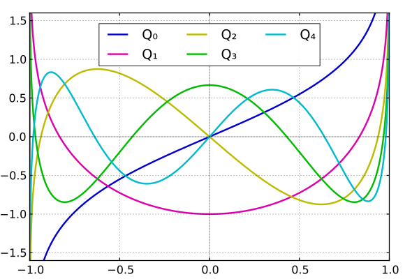
Legendre functions of the second kind ( $Q n$ )

As well as polynomial solutions, the Legendre equation has non-polynomial solutions represented by infinite series. These are the Legendre functions of the second kind, denoted by $Q n (x)$ .

displaystyle Q_n(x)=frac n!1cdot 3cdots (2n+1)left(x^-(n+1)+frac (n+1)(n+2)2(2n+3)x^-(n+3)+frac (n+1)(n+2)(n+3)(n+4)2cdot 4(2n+3)(2n+5)x^-(n+5)+cdots right)

The differential equation

displaystyle frac ddxleft(left(1-x^2right)frac ddxf(x)right)+n(n+1)f(x)=0

has the general solution

displaystyle f(x)=AP_n(x)+BQ_n(x),

where $A$ and $B$ are constants.

Notes

^ Arfken & Weber 2005, p.743

^ Legendre, A.-M. (1785) [1782]. "Recherches sur l'attraction des sphéroïdes homogènes". Mémoires de Mathématiques et de Physique, présentés à l'Académie Royale des Sciences, par divers savans, et lus dans ses Assemblées (PDF) (in French). X. Paris. pp. 411–435. Archived from the original (PDF) on 2009-09-20..mw-parser-output cite.citationfont-style:inherit.mw-parser-output .citation qquotes:"""""""'""'".mw-parser-output .citation .cs1-lock-free abackground:url("//upload.wikimedia.org/wikipedia/commons/thumb/6/65/Lock-green.svg/9px-Lock-green.svg.png")no-repeat;background-position:right .1em center.mw-parser-output .citation .cs1-lock-limited a,.mw-parser-output .citation .cs1-lock-registration abackground:url("//upload.wikimedia.org/wikipedia/commons/thumb/d/d6/Lock-gray-alt-2.svg/9px-Lock-gray-alt-2.svg.png")no-repeat;background-position:right .1em center.mw-parser-output .citation .cs1-lock-subscription abackground:url("//upload.wikimedia.org/wikipedia/commons/thumb/a/aa/Lock-red-alt-2.svg/9px-Lock-red-alt-2.svg.png")no-repeat;background-position:right .1em center.mw-parser-output .cs1-subscription,.mw-parser-output .cs1-registrationcolor:#555.mw-parser-output .cs1-subscription span,.mw-parser-output .cs1-registration spanborder-bottom:1px dotted;cursor:help.mw-parser-output .cs1-ws-icon abackground:url("//upload.wikimedia.org/wikipedia/commons/thumb/4/4c/Wikisource-logo.svg/12px-Wikisource-logo.svg.png")no-repeat;background-position:right .1em center.mw-parser-output code.cs1-codecolor:inherit;background:inherit;border:inherit;padding:inherit.mw-parser-output .cs1-hidden-errordisplay:none;font-size:100%.mw-parser-output .cs1-visible-errorfont-size:100%.mw-parser-output .cs1-maintdisplay:none;color:#33aa33;margin-left:0.3em.mw-parser-output .cs1-subscription,.mw-parser-output .cs1-registration,.mw-parser-output .cs1-formatfont-size:95%.mw-parser-output .cs1-kern-left,.mw-parser-output .cs1-kern-wl-leftpadding-left:0.2em.mw-parser-output .cs1-kern-right,.mw-parser-output .cs1-kern-wl-rightpadding-right:0.2em

^ Jackson, J. D. (1999). Classical Electrodynamics (3rd ed.). Wiley & Sons. p. 103. ISBN 978-0-471-30932-1.

^ Arfken & Weber 2005, p.753

^ 1895-1985., Szegő, Gábor, (1975). Orthogonal polynomials (4th ed.). Providence: American Mathematical Society. pp. 194 (Theorem 8.21.2). ISBN 0821810235. OCLC 1683237.

References

.mw-parser-output .refbeginfont-size:90%;margin-bottom:0.5em.mw-parser-output .refbegin-hanging-indents>ullist-style-type:none;margin-left:0.mw-parser-output .refbegin-hanging-indents>ul>li,.mw-parser-output .refbegin-hanging-indents>dl>ddmargin-left:0;padding-left:3.2em;text-indent:-3.2em;list-style:none.mw-parser-output .refbegin-100font-size:100%

Abramowitz, Milton; Stegun, Irene Ann, eds. (1983) [June 1964]. "Chapter 8". Handbook of Mathematical Functions with Formulas, Graphs, and Mathematical Tables. Applied Mathematics Series. 55 (Ninth reprint with additional corrections of tenth original printing with corrections (December 1972); first ed.). Washington D.C.; New York: United States Department of Commerce, National Bureau of Standards; Dover Publications. pp. 332, 773. ISBN 978-0-486-61272-0. LCCN 64-60036. MR 0167642. LCCN 65-12253. See also chapter 22.

Arfken, George B.; Weber, Hans J. (2005). Mathematical Methods for Physicists. Elsevier Academic Press. ISBN 0-12-059876-0.

Bayin, S. S. (2006). Mathematical Methods in Science and Engineering. Wiley. ch. 2. ISBN 978-0-470-04142-0.

Belousov, S. L. (1962). Tables of Normalized Associated Legendre Polynomials. Mathematical Tables. 18. Pergamon Press. ISBN 978-0-08-009723-7.

Courant, Richard; Hilbert, David (1953). Methods of Mathematical Physics. 1. New York, NY: Interscience. ISBN 978-0-471-50447-4.

Dunster, T. M. (2010), "Legendre and Related Functions", in Olver, Frank W. J.; Lozier, Daniel M.; Boisvert, Ronald F.; Clark, Charles W., NIST Handbook of Mathematical Functions, Cambridge University Press, ISBN 978-0521192255, MR 2723248

El Attar, Refaat (2009). Legendre Polynomials and Functions. CreateSpace. ISBN 978-1-4414-9012-4.

Koornwinder, Tom H.; Wong, Roderick S. C.; Koekoek, Roelof; Swarttouw, René F. (2010), "Orthogonal Polynomials", in Olver, Frank W. J.; Lozier, Daniel M.; Boisvert, Ronald F.; Clark, Charles W., NIST Handbook of Mathematical Functions, Cambridge University Press, ISBN 978-0521192255, MR 2723248

External links

A quick informal derivation of the Legendre polynomial in the context of the quantum mechanics of hydrogen

Hazewinkel, Michiel, ed. (2001) [1994], "Legendre polynomials", Encyclopedia of Mathematics, Springer Science+Business Media B.V. / Kluwer Academic Publishers, ISBN 978-1-55608-010-4

Wolfram MathWorld entry on Legendre polynomials

Dr James B. Calvert's article on Legendre polynomials from his personal collection of mathematics

The Legendre Polynomials by Carlyle E. Moore

Legendre Polynomials from Hyperphysics

[1] Arfken & Weber 2005, p.743

[2] Legendre, A.-M. (1785) [1782]. "Recherches sur l'attraction des sphéroïdes homogènes". Mémoires de Mathématiques et de Physique, présentés à l'Académie Royale des Sciences, par divers savans, et lus dans ses Assemblées (PDF) (in French). X. Paris. pp. 411–435. Archived from the original (PDF) on 2009-09-20..mw-parser-output cite.citationfont-style:inherit.mw-parser-output .citation qquotes:"""""""'""'".mw-parser-output .citation .cs1-lock-free abackground:url("//upload.wikimedia.org/wikipedia/commons/thumb/6/65/Lock-green.svg/9px-Lock-green.svg.png")no-repeat;background-position:right .1em center.mw-parser-output .citation .cs1-lock-limited a,.mw-parser-output .citation .cs1-lock-registration abackground:url("//upload.wikimedia.org/wikipedia/commons/thumb/d/d6/Lock-gray-alt-2.svg/9px-Lock-gray-alt-2.svg.png")no-repeat;background-position:right .1em center.mw-parser-output .citation .cs1-lock-subscription abackground:url("//upload.wikimedia.org/wikipedia/commons/thumb/a/aa/Lock-red-alt-2.svg/9px-Lock-red-alt-2.svg.png")no-repeat;background-position:right .1em center.mw-parser-output .cs1-subscription,.mw-parser-output .cs1-registrationcolor:#555.mw-parser-output .cs1-subscription span,.mw-parser-output .cs1-registration spanborder-bottom:1px dotted;cursor:help.mw-parser-output .cs1-ws-icon abackground:url("//upload.wikimedia.org/wikipedia/commons/thumb/4/4c/Wikisource-logo.svg/12px-Wikisource-logo.svg.png")no-repeat;background-position:right .1em center.mw-parser-output code.cs1-codecolor:inherit;background:inherit;border:inherit;padding:inherit.mw-parser-output .cs1-hidden-errordisplay:none;font-size:100%.mw-parser-output .cs1-visible-errorfont-size:100%.mw-parser-output .cs1-maintdisplay:none;color:#33aa33;margin-left:0.3em.mw-parser-output .cs1-subscription,.mw-parser-output .cs1-registration,.mw-parser-output .cs1-formatfont-size:95%.mw-parser-output .cs1-kern-left,.mw-parser-output .cs1-kern-wl-leftpadding-left:0.2em.mw-parser-output .cs1-kern-right,.mw-parser-output .cs1-kern-wl-rightpadding-right:0.2em

[3] Jackson, J. D. (1999). Classical Electrodynamics (3rd ed.). Wiley & Sons. p. 103. ISBN 978-0-471-30932-1.

[4] Arfken & Weber 2005, p.753

[5] 1895-1985., Szegő, Gábor, (1975). Orthogonal polynomials (4th ed.). Providence: American Mathematical Society. pp. 194 (Theorem 8.21.2). ISBN 0821810235. OCLC 1683237.

搜尋此網誌