Xrthnty

Viscosity
	; A simulation of liquids with different viscosities. The liquid on the right has higher viscosity than the liquid on the left.;
Common symbols	; η, μ;
Derivations from; other quantities	μ = G·t

The viscosity of a fluid is the measure of its resistance to gradual deformation by shear stress or tensile stress.^[1] For liquids, it corresponds to the informal concept of "thickness": for example, syrup has a higher viscosity than water.^[2]

Viscosity is the property of a fluid which opposes the relative motion between two surfaces of the fluid that are moving at different velocities. In simple terms, viscosity means friction between the molecules of fluid. When the fluid is forced through a tube, the particles which compose the fluid generally move more quickly near the tube's axis and more slowly near its walls; therefore some stress (such as a pressure difference between the two ends of the tube) is needed to overcome the friction between particle layers to keep the fluid moving. For a given velocity pattern, the stress required is proportional to the fluid's viscosity.

A fluid that has no resistance to shear stress is known as an ideal or inviscid fluid. Zero viscosity is observed only at very low temperatures in superfluids. Otherwise, the second law of thermodynamics requires all fluids to have positive viscosity;^[3] such fluids are technically said to be viscous or viscid. A fluid with a relatively high viscosity, such as pitch, may appear to be a solid.

.mw-parser-output .toclimit-2 .toclevel-1 ul,.mw-parser-output .toclimit-3 .toclevel-2 ul,.mw-parser-output .toclimit-4 .toclevel-3 ul,.mw-parser-output .toclimit-5 .toclevel-4 ul,.mw-parser-output .toclimit-6 .toclevel-5 ul,.mw-parser-output .toclimit-7 .toclevel-6 uldisplay:none

Etymology

The word "viscosity" is derived from the Latin "viscum", meaning mistletoe and also a viscous glue made from mistletoe berries.^[4]

Definition

Simple definition

Illustration of a planar Couette flow. Since the shearing flow is opposed by friction between adjacent layers of fluid (which are in relative motion), a force is required to sustain the motion of the upper plate. The relative strength of this force is a measure of the fluid's viscosity.

In a general parallel flow, the shear stress is proportional to the gradient of the velocity.

In materials science and engineering, one is often interested in understanding the forces involved in the deformation of a material. In other words, one wishes to know what stresses arise in a material as the result of some given deformation. For instance, if the material were a simple spring, the answer would be given by Hooke's law, which says that the force experienced by a spring is proportional to the distance displaced from equilibrium. Stresses which can be attributed to the deformation of a material from some rest state are called elastic stresses. In other materials, stresses are present which can be attributed to the rate of change of the deformation over time, rather than the magnitude of the deformation. These are called viscous stresses. For instance, in a fluid like water, the stresses which arise from shearing the fluid are clearly independent of the distance the fluid has been sheared; instead, they depend on how quickly the shearing occurs.

Viscosity is the material property which relates the viscous stresses in a material to the rate of change of a deformation (the strain rate). Although it applies to general flows, it is easiest to visualize and define in a simple shearing flow, such as a planar Couette flow.

In the Couette flow, a fluid is trapped between two infinitely large plates, one fixed and one in parallel motion at constant speed $u$ (see illustration to the right). If the speed of the top plate is low enough (to avoid turbulence), then in steady state the fluid particles move parallel to it, and their speed varies from $displaystyle 0$ at the bottom to $u$ at the top.^[5] Each layer of fluid moves faster than the one just below it, and friction between them gives rise to a force resisting their relative motion. In particular, the fluid applies on the top plate a force in the direction opposite to its motion, and an equal but opposite force on the bottom plate. An external force is therefore required in order to keep the top plate moving at constant speed.

In many fluids, the flow velocity is observed to vary linearly from zero at the bottom to $u$ at the top. Moreover, the magnitude $F$ of the force acting on the top plate is found to be proportional to the speed $u$ and the area $A$ of each plate, and inversely proportional to their separation $y$ :

F=mu Afrac uy.

The proportionality factor $mu$ is the viscosity of the fluid, with units of $displaystyle textPacdot texts$ (pascal-second). The ratio $u/y$ is called the rate of shear deformation or shear velocity, and is the derivative of the fluid speed in the direction perpendicular to the plates (see illustrations to the right). If the velocity does not vary linearly with $y$ , then the appropriate generalization is

tau =mu frac partial upartial y,

where $displaystyle tau =F/A$ , and $displaystyle partial u/partial y$ is the local shear velocity. This expression is referred to as Newton's law of viscosity. In shearing flows with planar symmetry, it is what defines $mu$ . It is a special case of the general definition of viscosity (see below), which can be expressed in coordinate-free form.

Use of the Greek letter mu ( $mu$ ) for the viscosity is common among mechanical and chemical engineers, as well as physicists.^[6]^[7]^[8] However, the Greek letter eta ( $eta$ ) is also used by chemists, physicists, and the IUPAC.^[9] The viscosity $mu$ is sometimes also referred to as the shear viscosity. However, at least one author discourages the use of this terminology, noting that $mu$ can be appear in nonshearing flows in addition to shearing flows.^[10]

General definition

In very general terms, the viscous stresses in a fluid are defined as those resulting from the relative velocity of different fluid particles. As such, the viscous stresses must depend on spatial gradients of the flow velocity. If the velocity gradients are small, then to a first approximation the viscous stresses depend only on the first derivatives of the velocity.^[11] (For Newtonian fluids, this is also a linear dependence.) In Cartesian coordinates, the general relationship can then be written as

displaystyle tau _ij=sum _ksum _lmu _ijklfrac partial v_kpartial r_l,

where $displaystyle mu _ijkl$ is a viscosity tensor that maps the strain rate tensor $displaystyle partial v_k/partial r_l$ onto the viscous stress tensor $tau _ij$ .^[12] Since the indices in this expression can vary from 1 to 3, there are 81 "viscosity coefficients" $displaystyle mu _ijkl$ in total. However, due to spatial symmetries these coefficients are not all independent. For instance, for isotropic Newtonian fluids, the 81 coefficients can be reduced to 2 independent parameters. The most usual decomposition yields the standard (scalar) viscosity $mu$ and the bulk viscosity $kappa$ :

displaystyle mathbf tau =mu left[nabla mathbf v +(nabla mathbf v )^dagger right]-left(frac 23mu -kappa right)(nabla cdot mathbf v )mathbf delta ,

where $displaystyle mathbf delta$ is the unit tensor, and the dagger $dagger$ denotes the transpose.^[13]^[14] This equation can be thought of as a generalized form of Newton's law of viscosity.

The bulk viscosity expresses a type of internal friction that resists the shearless compression or expansion of a fluid. Knowledge of $kappa$ is frequently not necessary in fluid dynamics problems. For example, incompressible liquids satisfy $nabla cdot mathbf v=0$ and so the term containing $kappa$ is absent. Moreover, $kappa$ is often assumed to be negligible for gases since it is $displaystyle 0$ in a monoatomic ideal gas.^[13] One situation in which $kappa$ can be important is the calculation of energy loss in sound and shock waves, described by Stokes' law of sound attenuation, since these phenomena involve rapid expansions and compressions.

It is worth emphasizing that the above expressions are not fundamental laws of nature, but rather definitions of viscosity. As such, their utility for any given material, as well as means for measuring or calculating the viscosity, must be established using separate and independent means.

Dynamic and kinematic viscosity

In fluid dynamics, it is common to work in terms of the kinematic viscosity (also called "momentum diffusivity"), defined as the ratio of the viscosity $μ$ to the density of the fluid $ρ$ . It is usually denoted by the Greek letter nu ( $ν$ ) and has units $displaystyle mathrm (length)^2/time$ :

nu =frac mu rho

.

Consistent with this nomenclature, the viscosity $mu$ is frequently called the dynamic viscosity.

Momentum transport

Transport theory provides an alternate interpretation of viscosity in terms of momentum transport: viscosity is the material property which characterizes momentum transport within a fluid, just as thermal conductivity characterizes heat transport, and (mass) diffusivity characterizes mass transport.^[15] To see this, note that in Newton's law of viscosity, $displaystyle tau =mu (partial u/partial y)$ , the shear stress $tau$ has units equivalent to a momentum flux, i.e. momentum per unit time per unit area. Thus, $tau$ can be interpreted as specifying the flow of momentum in the $y$ direction from one fluid layer to the next. Per Newton's law of viscosity, this momentum flow occurs across a velocity gradient, and the magnitude of the corresponding momentum flux is determined by the viscosity.

The analogy with heat and mass transfer can be made explicit. Just as heat flows from high temperature to low temperature and mass flows from high density to low density, momentum flows from high velocity to low velocity. These behaviors are all described by compact expressions, called constitutive relations, whose one-dimensional forms are given here:

displaystyle beginalignedmathbf J &=-Dfrac partial rho partial xqquad ;;;,text(Fick's law of diffusion)\mathbf q &=-k_tfrac partial Tpartial xqquad ;;,text(Fourier's law of heat conduction)\tau &=mu frac partial upartial yqquad qquad text(Newton's law of viscosity)\endaligned

where $rho$ is the density, $mathbf J$ and $mathbf q$ are the mass and heat fluxes, and $D$ and $k_t$ are the mass diffusivity and thermal conductivity.^[16]

The fact that mass, momentum, and energy (heat) transport are among the most relevant processes in continuum mechanics is not a coincidence: these are among the few physical quantities that are conserved at the microscopic level in interparticle collisions. Thus, rather than being dictated by the fast and complex microscopic interaction timescale, their dynamics occurs on macroscopic timescales, as described by the various equations of transport theory and hydrodynamics.

Newtonian and non-Newtonian fluids

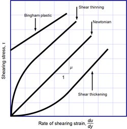
Viscosity, the slope of each line, varies among materials.

Newton's law of viscosity is a constitutive equation (like Hooke's law, Fick's law, and Ohm's law): it is not a fundamental law of nature but an approximation that holds in some materials and fails in others.

A fluid that behaves according to Newton's law, with a viscosity $μ$ that is independent of the stress, is said to be Newtonian. Gases, water, and many common liquids can be considered Newtonian in ordinary conditions and contexts. There are many non-Newtonian fluids that significantly deviate from that law in some way or other. For example:

Shear-thickening liquids, whose viscosity increases with the rate of shear strain.

Shear-thinning liquids, whose viscosity decreases with the rate of shear strain.

Thixotropic liquids, that become less viscous over time when shaken, agitated, or otherwise stressed.

Rheopectic (dilatant) liquids, that become more viscous over time when shaken, agitated, or otherwise stressed.

Bingham plastics that behave as a solid at low stresses but flow as a viscous fluid at high stresses.

Shear-thinning liquids are very commonly, but misleadingly, described as thixotropic.^[17]

Even for a Newtonian fluid, the viscosity usually depends on its composition and temperature. For gases and other compressible fluids, it depends on temperature and varies very slowly with pressure.

The viscosity of some fluids may depend on other factors. A magnetorheological fluid, for example, becomes thicker when subjected to a magnetic field, possibly to the point of behaving like a solid.

In solids

The viscous forces that arise during fluid flow must not be confused with the elastic forces that arise in a solid in response to shear, compression or extension stresses. While in the latter the stress is proportional to the amount of shear deformation, in a fluid it is proportional to the rate of deformation over time. (For this reason, Maxwell used the term fugitive elasticity for fluid viscosity.)

However, many liquids (including water) will briefly react like elastic solids when subjected to sudden stress. Conversely, many "solids" (even granite) will flow like liquids, albeit very slowly, even under arbitrarily small stress.^[18] Such materials are therefore best described as possessing both elasticity (reaction to deformation) and viscosity (reaction to rate of deformation); that is, being viscoelastic.

Indeed, some authors have claimed that amorphous solids, such as glass and many polymers, are actually liquids with a very high viscosity (greater than 10¹² Pa·s).
^[19] However, other authors dispute this hypothesis, claiming instead that there is some threshold for the stress, below which most solids will not flow at all,^[20] and that alleged instances of glass flow in window panes of old buildings are due to the crude manufacturing process of older eras rather than to the viscosity of glass.^[21]

Viscoelastic solids may exhibit both shear viscosity and bulk viscosity. The extensional viscosity is a linear combination of the shear and bulk viscosities that describes the reaction of a solid elastic material to elongation. It is widely used for characterizing polymers.

In geology, earth materials that exhibit viscous deformation at least three orders of magnitude greater than their elastic deformation are sometimes called rheids.^[22]

Measurement

Viscosity is measured with various types of viscometers and rheometers. A rheometer is used for those fluids that cannot be defined by a single value of viscosity and therefore require more parameters to be set and measured than is the case for a viscometer. Close temperature control of the fluid is essential to acquire accurate measurements, particularly in materials like lubricants, whose viscosity can double with a change of only 5 °C.

For some fluids, the viscosity is constant over a wide range of shear rates (Newtonian fluids). The fluids without a constant viscosity (non-Newtonian fluids) cannot be described by a single number. Non-Newtonian fluids exhibit a variety of different correlations between shear stress and shear rate.

One of the most common instruments for measuring kinematic viscosity is the glass capillary viscometer.

In coating industries, viscosity may be measured with a cup in which the efflux time is measured. There are several sorts of cup – such as the Zahn cup and the Ford viscosity cup – with the usage of each type varying mainly according to the industry. The efflux time can also be converted to kinematic viscosities (centistokes, cSt) through the conversion equations.^[23]

Also used in coatings, a Stormer viscometer uses load-based rotation in order to determine viscosity. The viscosity is reported in Krebs units (KU), which are unique to Stormer viscometers.

Vibrating viscometers can also be used to measure viscosity. Resonant, or vibrational viscometers work by creating shear waves within the liquid. In this method, the sensor is submerged in the fluid and is made to resonate at a specific frequency. As the surface of the sensor shears through the liquid, energy is lost due to its viscosity. This dissipated energy is then measured and converted into a viscosity reading. A higher viscosity causes a greater loss of energy.^{[citation needed]}

Extensional viscosity can be measured with various rheometers that apply extensional stress.

Volume viscosity can be measured with an acoustic rheometer.

Apparent viscosity is a calculation derived from tests performed on drilling fluid used in oil or gas well development. These calculations and tests help engineers develop and maintain the properties of the drilling fluid to the specifications required.

Units

The SI unit of dynamic viscosity is Pa·s or kg·m⁻¹·s⁻¹. The cgs unit is called the poise^[24] (P), named after Jean Léonard Marie Poiseuille. It is commonly expressed, particularly in ASTM standards, as centipoise (cP) since the latter is equal to the SI multiple millipascal seconds (mPa·s).

The SI unit of kinematic viscosity is m²/s, whereas the cgs unit for kinematic viscosity is the stokes (St), named after Sir George Gabriel Stokes.^[25] It is sometimes expressed in terms of centistokes (cSt). In U.S. usage, stoke is sometimes used as the singular form.

The reciprocal of viscosity is fluidity, usually symbolized by $displaystyle phi =1/mu$ or $displaystyle F=1/mu$ , depending on the convention used, measured in reciprocal poise (P⁻¹, or cm·s·g⁻¹), sometimes called the rhe. Fluidity is seldom used in engineering practice.

Nonstandard units include the reyn, a British unit of dynamic viscosity.^{[citation needed]} In the automotive industry the viscosity index is used to describe the change of viscosity with temperature.

At one time the petroleum industry relied on measuring kinematic viscosity by means of the Saybolt viscometer, and expressing kinematic viscosity in units of Saybolt universal seconds (SUS).^[26] Other abbreviations such as SSU (Saybolt seconds universal) or SUV (Saybolt universal viscosity) are sometimes used. Kinematic viscosity in centistokes can be converted from SUS according to the arithmetic and the reference table provided in ASTM D 2161.^[27]

Molecular origins

In general, the viscosity of a system depends in detail on how the molecules constituting the system interact. There are no simple but correct expressions for the viscosity of a fluid. The simplest exact expressions are the Green–Kubo relations for the linear shear viscosity or the transient time correlation function expressions derived by Evans and Morriss in 1985.^[28] Although these expressions are each exact, calculating the viscosity of a dense fluid using these relations currently requires the use of molecular dynamics computer simulations. On the other hand, much more progress can be made for a dilute gas. Even elementary assumptions about how gas molecules move and interact lead to a basic understanding of the molecular origins of viscosity. More sophisticated treatments can be constructed by systematically coarse-graining the equations of motion of the gas molecules. An example of such a treatment is Chapman–Enskog theory, which derives expressions for the viscosity of a dilute gas from the Boltzmann equation.^[29]

Momentum transport in gases is generally mediated by discrete molecular collisions, and in liquids by attractive forces which bind molecules close together.^[30] Because of this, the dynamic viscosities of liquids are typically much larger than those of gases.

Gases

Elementary calculation of viscosity for a dilute gas

Consider a dilute gas moving parallel to the $x$ -axis with velocity $u(y)$ that depends only on the $y$ coordinate. To simplify the discussion, the gas is assumed to have uniform temperature and density.

Under these assumptions, the $x$ velocity of a molecule passing through $y=0$ is equal to whatever velocity that molecule had when its mean free path $lambda$ began. Because $lambda$ is typically small compared with macroscopic scales, the average $x$ velocity of such a molecule has the form

displaystyle u(0)pm alpha lambda frac dudy(0)

,

where $alpha$ is a numerical constant on the order of $1$ . (Some authors estimate $displaystyle alpha =2/3$ ;^[30]^[31] on the other hand, a more careful calculation for rigid elastic spheres gives $displaystyle alpha simeq 0.998$ .) Now, because half the molecules on either side are moving towards $y=0$ , and doing so on average with half the average moleculer speed $displaystyle (8k_textBT/pi m)^1/2$ , the momentum flux from either side is

displaystyle frac 14rho cdot sqrt frac 8k_textBTpi mcdot left(u(0)pm alpha lambda frac dudy(0)right).

The net momentum flux at $y=0$ is the difference of the two:

displaystyle -frac 12rho cdot sqrt frac 8k_textBTpi mcdot alpha lambda frac dudy(0).

According to the definition of viscosity, this momentum flux should be equal to $displaystyle -mu frac dudy(0)$ , which leads to

displaystyle mu =alpha rho lambda sqrt frac 2k_textBTpi m.

Viscosity in gases arises principally from the molecular diffusion that transports momentum between layers of flow. An elementary calculation for a dilute gas at temperature $T$ and density $rho$ gives

displaystyle mu =alpha rho lambda sqrt frac 2k_textBTpi m,

where $k_textB$ is the Boltzmann constant, $m$ the molecular mass, and $alpha$ a numerical constant on the order of $1$ . The quantity $lambda$ , the mean free path, measures the average distance a molecule travels between collisions. Even without a priori knowledge of $alpha$ , this expression has interesting implications. In particular, since $lambda$ is typically inversely proportional to density and increases with temperature, $mu$ itself should increase with temperature and be independent of density at fixed temperature. In fact, both of these predictions persist in more sophisticated treatments, and accurately describe experimental observations. Note that this behavior runs counter to common intuition regarding liquids, for which viscosity typically decreases with temperature.^[30]^[31]

For rigid elastic spheres of diameter $sigma$ , $lambda$ can be computed, giving

displaystyle mu =frac alpha pi ^3/2frac sqrt k_textBmTsigma ^2.

In this case $lambda$ is independent of temperature, so $displaystyle mu propto T^1/2$ . For more complicated molecular models, however, $lambda$ depends on temperature in a non-trivial way, and simple kinetic arguments as used here are inadequate. More fundamentally, the notion of a mean free path becomes imprecise for particles that interact over a finite range, which limits the usefulness of the concept for describing real-world gases.^[32]

Chapman–Enskog theory

A technique developed by Sydney Chapman and David Enskog in the early 1900s allows a more refined calculation of $mu$ .^[29] It is based on the Boltzmann equation, which provides a systematic statistical description of a dilute gas in terms of intermolecular interactions.^[33] As such, their technique allows accurate calculation of $mu$ for more realistic molecular models, such as those incorporating intermolecular attraction rather than just hard-core repulsion.

It turns out that a more realistic modeling of interactions is essential for accurate prediction of the temperature dependence of $mu$ , which experiments show increases more rapidly than the $T^1/2$ trend predicted for rigid elastic spheres.^[30] Indeed, the Chapman–Enskog analysis shows that the predicted temperature dependence can be tuned by varying the parameters in various molecular models. A simple example is the Sutherland model,^[34] which describes rigid elastic spheres with weak mutual attraction. In such a case, the attractive force can be treated perturbatively, which leads to a particularly simple expression for $mu$ :

displaystyle mu =frac 516sigma ^2left(frac k_textBmTpi right)^1/2left(1+frac STright)^-1,

where $S$ is independent of temperature, being determined only by the parameters of the intermolecular attraction. To connect with experiment, it is convenient to rewrite as

displaystyle mu =mu _0left(frac TT_0right)^3/2frac T_0+ST+S,

where $mu _0$ is the viscosity at temperature $T_0$ . If $mu$ is known from experiments at $T=T_0$ and at least one other temperature, then $S$ can be calculated. It turns out that expressions for $mu$ obtained in this way are accurate for a number of gases over a sizable range of temperatures. On the other hand, Chapman and Cowling^[29] argue that this success does not imply that molecules actually interact according to the Sutherland model. Rather, they interpret the prediction for $mu$ as a simple interpolation which is valid for some gases over fixed ranges of temperature, but otherwise does not provide a picture of intermolecular interactions which is fundamentally correct and general. Slightly more sophisticated models, such as the Lennard–Jones potential, may provide a better picture, but only at the cost of a more opaque dependence on temperature. In some systems the assumption of spherical symmetry must be abandoned as well, as is the case for vapors with highly polar molecules like H₂O.^[35]^[36]

Liquids

Play media

Video showing three liquids with different viscosities

Play media

Experiment showing the behavior of a viscous fluid with blue dye for visibility

In contrast with gases, there is no simple yet accurate picture for the molecular origins of viscosity in liquids.

At the simplest level of description, the relative motion of adjacent layers in a liquid is opposed primarily by attractive molecular forces
acting across the layer boundary. In this picture, one (correctly) expects viscosity to decrease with increasing temperature. This is because
increasing temperature increases the random thermal motion of the molecules, which makes it easier for them to overcome their attractive interactions.^[37]

Building on this visualization, a simple theory can be constructed in analogy with the discrete structure of a solid: groups of molecules in a liquid
are visualized as forming "cages" which surround and enclose single molecules.^[38] These cages can be occupied or unoccupied, and
stronger molecular attraction corresponds to stronger cages.
Due to random thermal motion, a molecule "hops" between cages at a rate which varies inversely with the strength of molecular attractions. In equilibrium these "hops" are not biased in any direction.
On the other hand, in order for two adjacent layers to move relative to each other, the "hops" must be biased in the direction
of the relative motion. The force required to sustain this directed motion can be estimated for a given shear rate, leading to

$displaystyle mu approx frac N_AhVoperatorname exp left(3.8frac T_bTright),$

(1)

where $N_A$ is the Avogadro constant, $h$ is the Planck constant, $V$ is the volume of a mole of liquid, and $T_b$ is the normal boiling point. This result has the same form as the widespread and accurate empirical relation

$displaystyle mu =Ae^frac BT,$

(2)

where $A$ and $B$ are constants fit from data.^[38]^[39] One the other hand, several authors express caution with respect to this model.
Errors as large as 30% can be encountered using equation (1), compared with fitting equation (2) to experimental data.^[38] More fundamentally, the physical assumptions underlying equation (1) have been extensively criticized.^[40] It has also been argued that the exponential dependence in equation (1) does not necessarily describe experimental observations more accurately than simpler, non-exponential expressions.^[41]^[42]

In light of these shortcomings, the development of a less ad-hoc model is a matter of practical interest.
Foregoing simplicity in favor of precision, it is possible to write rigorous expressions for viscosity starting from the fundamental equations of motion for molecules. A classic example
of this approach is Irving-Kirkwood theory.^[43] On the other hand, such expressions
are given as averages over multiparticle correlation functions and are therefore difficult to apply in practice.

In general, empirically derived expressions (based on existing viscosity measurements) appear to be the only consistently reliable means of calculating viscosity in liquids.^[44]

Mixtures, blends, and suspensions

Gaseous mixtures

The same molecular-kinetic picture of a single component gas can also be applied to a gaseous mixture. For instance, in the Chapman-Enskog approach the viscosity $displaystyle mu _textmix$ of a binary mixture of gases can be written in terms of the individual component viscosities $displaystyle mu _1,2$ , their respective volume fractions, and the intermolecular interactions.^[45] As for the single-component gas, the dependence of $displaystyle mu _textmix$ on the parameters of the intermolecular interactions enters through various collisional integrals which may not be expressible in terms of elementary functions. To obtain usable expressions for $displaystyle mu _textmix$ which reasonably match experimental data, the collisional integrals typically must be evaluated using some combination of analytic calculation and empirical fitting. An example of such a procedure is the Sutherland approach for the single-component gas, discussed above.

Blends of liquids

As for pure liquids, the viscosity of a blend of liquids is difficult to predict from molecular principles. One method is to extend the molecular "cage" theory presented above for a pure liquid. This can be done with varying levels of sophistication. One useful expression resulting from such an analysis is the Lederer-Roegiers equation for a binary mixture:

displaystyle mu _textblend=frac x_1x_1+alpha x_2ln mu _1+frac alpha x_2x_1+alpha x_2ln mu _2,

where $alpha$ is an empirical parameter, and $displaystyle x_1,2$ and $displaystyle mu _1,2$ are the respective mole fractions and viscosities of the component liquids.^[46]

Since blending is an important process in the lubricating and oil industries, a variety of empirical and propriety equations exist for predicting the viscosity of a blend, besides those stemming directly from molecular theory.^[46]

Suspensions

In a suspension of solid particles (e.g. micron-size spheres suspended in oil), an effective viscosity $displaystyle mu _texteff$ can be defined in terms of stress and strain components which are averaged over a volume large compared with the distance between the suspended particles, but small with respect to macroscopic dimensions.^[47] Such suspensions generally exhibit non-Newtonian behavior. However, for dilute systems in steady flows, the behavior is Newtonian and expressions for $displaystyle mu _texteff$ can be derived directly from the particle dynamics. In a very dilute system, with volume fraction $displaystyle phi lesssim 0.02$ , interactions between the suspended particles can be ignored. In such a case one can explicitly calculate the flow field around each particle independently, and combine the results to obtain $displaystyle mu _texteff$ . For spheres, this results in the Einstein equation:

$displaystyle mu _texteff=mu _0left(1+frac 52phi right),$

where $mu _0$ is the viscosity of the suspending liquid. The linear dependence on $phi$ is a direct consequence of neglecting interparticle interactions; in general, one will have:

$displaystyle mu _texteff=mu _0left(1+Bphi right),$

where the coefficient $B$ may depend on the particle shape (e.g. spheres, rods, disks).^[48] Perhaps surprisingly, in the century since its introduction the coefficient for spheres, $displaystyle B=5/2$ , has not been conclusively pinned down by experiments, with various experiments finding values in the range $displaystyle 1.5lesssim Blesssim 5$ .^[49] This deficiency has been attributed to difficulty in controlling experimental conditions.^[50]

In denser suspensions, $displaystyle mu _texteff$ acquires a nonlinear dependence on $phi$ , which indicates the importance of interparticle interactions. Various analytical and semi-empirical schemes exist for capturing this regime. At the most basic level, a term quadratic in $phi$ is added to $displaystyle mu _texteff$ :

$displaystyle mu _texteff=mu _0left(1+Bphi +B_1phi ^2right),$

and the coefficient $B_1$ is fit from experimental data or approximated from the microscopic theory. In general, however, one should be cautious in applying such simple formulas since non-Newtonian behavior appears in dense suspensions ( $displaystyle phi gtrsim 0.25$ for spheres),^[49] or in suspensions of elongated or flexible particles.^[51]

A distinction must be made between a suspension of solid particles, described above, and an emulsion. The latter is a suspension of tiny droplets, which themselves may exhibit internal circulation. The presence of internal circulation can noticeably decrease the observed effective viscosity, and different theoretical or semi-empirical models must be used.^[52]

Amorphous materials

Common glass viscosity curves^[53]

In the high and low temperature limits, viscous flow in amorphous materials (e.g. in glasses and melts)^[54]^[55]^[56] has the Arrhenius form:

displaystyle mu =Ae^frac QRT,

where $Q$ is a relevant activation energy, given in terms of molecular parameters; $T$ is temperature; $R$ is the molar gas constant; and $A$ is approximately a constant. The activation energy $Q$ takes a different value depending on whether the high or low temperature limit is being considered: it changes from a high value $Q H$ at low temperatures (in the glassy state) to a low value $Q L$ at high temperatures (in the liquid state).

Common logarithm of viscosity against temperature for B₂O₃, showing two regimes

For intermediate temperatures, $Q$ varies nontrivially with temperature and the simple Arrhenius form fails. On the other hand, the two-exponential equation

displaystyle mu =ATexp left(frac BRTright)left[1+Cexp left(frac DRTright)right],

where $A$ , $B$ , $C$ , $D$ are all constants, provides a good fit to experimental data over the entire range of temperatures, while at the same time reducing to the correct Arrhenius form in the low and high temperature limits. Besides being a convenient fit to data, the expression can also be derived from various theoretical models of amorphous materials at the atomic level.^[56]

Eddy viscosity

In the study of turbulence in fluids, a common practical strategy for calculation is to ignore the small-scale vortices (or eddies) in the motion and to calculate a large-scale motion with an eddy viscosity that characterizes the transport and dissipation of energy in the smaller-scale flow (see large eddy simulation).^[57]^[58] Values of eddy viscosity used in modeling ocean circulation may be from 7004500000000000000♠5×10⁴ to 7006100000000000000♠1×10⁶ Pa·s depending upon the resolution of the numerical grid.^{[citation needed]}

Selected substances

In the University of Queensland pitch drop experiment, pitch has been dripping slowly through a funnel since 1927, at a rate of one drop roughly every decade. In this way the viscosity of pitch has been determined to be approximately 230 billion (7011229999999999999♠2.3×10¹¹) times that of water.^[59]

Observed values of viscosity vary over several orders of magnitude, even for common substances. For instance, a 70% sucrose (sugar) solution has a viscosity over 400 times that of water, and 26000 times that of air.^[60] More dramatically, pitch has been estimated to have a viscosity 230 billion times that of water.^[59]

Water

The viscosity of water is about 0.89 mPa·s at room temperature (25 °C). As a function of temperature, the viscosity can be estimated using the semi-empirical relation:

displaystyle mu =Atimes 10^B/(T-C),

where $A$ = 6995241400000000000♠2.414×10⁻⁵ Pa·s, $B$ = 247.8 K, and $C$ = 140 K.^{[citation needed]}

Experimentally determined values of the viscosity at various temperatures are given below.

Viscosity of water
at various temperatures^[60]
Temperature (°C)	Viscosity (mPa·s)
10	1.3059
20	1.0016
30	0.79722
50	0.54652
70	0.40355
90	0.31417

Air

Under standard atmospheric conditions (25 °C and pressure of 1 bar), the viscosity of air is 18.5 μPa·s, roughly 50 times smaller than the viscosity of water at the same temperature. Except at very high pressure, the viscosity of air depends mostly on the temperature.

Other common substances

Honey being drizzled

Substance	Viscosity (cPa·s)	Temperature (°C)
Whole milk^[61]	2.12	20
Olive oil^[61]	56.2	26
Honey^[62]	$approx$ 2000-10000	20
Ketchup^[a]^[63]	$approx$ 5000-20000	25
Peanut butter^[a]^[64]	$approx$ 10⁴-10⁶
Pitch^[59]	7011229999999999999♠2.3×10¹¹	10-30 (variable)

^ ^a^b These materials are highly non-Newtonian.

References

^ "viscosity". Merriam-Webster Dictionary..mw-parser-output cite.citationfont-style:inherit.mw-parser-output qquotes:"""""""'""'".mw-parser-output code.cs1-codecolor:inherit;background:inherit;border:inherit;padding:inherit.mw-parser-output .cs1-lock-free abackground:url("//upload.wikimedia.org/wikipedia/commons/thumb/6/65/Lock-green.svg/9px-Lock-green.svg.png")no-repeat;background-position:right .1em center.mw-parser-output .cs1-lock-limited a,.mw-parser-output .cs1-lock-registration abackground:url("//upload.wikimedia.org/wikipedia/commons/thumb/d/d6/Lock-gray-alt-2.svg/9px-Lock-gray-alt-2.svg.png")no-repeat;background-position:right .1em center.mw-parser-output .cs1-lock-subscription abackground:url("//upload.wikimedia.org/wikipedia/commons/thumb/a/aa/Lock-red-alt-2.svg/9px-Lock-red-alt-2.svg.png")no-repeat;background-position:right .1em center.mw-parser-output .cs1-subscription,.mw-parser-output .cs1-registrationcolor:#555.mw-parser-output .cs1-subscription span,.mw-parser-output .cs1-registration spanborder-bottom:1px dotted;cursor:help.mw-parser-output .cs1-hidden-errordisplay:none;font-size:100%.mw-parser-output .cs1-visible-errorfont-size:100%.mw-parser-output .cs1-subscription,.mw-parser-output .cs1-registration,.mw-parser-output .cs1-formatfont-size:95%.mw-parser-output .cs1-kern-left,.mw-parser-output .cs1-kern-wl-leftpadding-left:0.2em.mw-parser-output .cs1-kern-right,.mw-parser-output .cs1-kern-wl-rightpadding-right:0.2em

^ Symon, Keith (1971). Mechanics (3rd ed.). Addison-Wesley. ISBN 978-0-201-07392-8.

^ Balescu, Radu (1975), Equilibrium and Nonequilibrium Statistical Mechanics, John Wiley & Sons, pp. 428–429, ISBN 978-0-471-04600-4

^ "viscous". Etymonline.com. Retrieved 2010-09-14.

^ Jan Mewis; Norman J. Wagner (2012). Colloidal Suspension Rheology. Cambridge University Press. p. 19. ISBN 978-0-521-51599-3.

^ Streeter, Victor Lyle; Wylie, E. Benjamin; Bedford, Keith W. (1998). Fluid Mechanics. McGraw-Hill. ISBN 978-0-07-062537-2.

^ Holman, J. P. (2002). Heat Transfer. McGraw-Hill. ISBN 978-0-07-122621-9.

^ Incropera, Frank P.; DeWitt, David P. (2007). Fundamentals of Heat and Mass Transfer. Wiley. ISBN 978-0-471-45728-2.

^ Nič, Miloslav; Jirát, Jiří; Košata, Bedřich; Jenkins, Aubrey, eds. (1997). "dynamic viscosity, η". IUPAC Compendium of Chemical Terminology. Oxford: Blackwell Scientific Publications. doi:10.1351/goldbook. ISBN 978-0-9678550-9-7.

^ Bird, R. Byron; Stewart, Warren E.; Lightfoot, Edwin N. (2007), Transport Phenomena (2nd ed.), John Wiley & Sons, Inc., p. 19, ISBN 978-0-470-11539-8

^ Landau, L.D.; Lifshitz, E.M. (1987), Fluid Mechanics (2nd ed.), Pergamon Press, pp. 44–45, ISBN 0-08-033933-6

^ Bird, Steward, & Lightfoot, p. 18 (Note that this source uses a alternate sign convention, which has been reversed here.)

^ ^a^b Bird, Steward, & Lightfoot, p. 19

^ Landau & Lifshitz p. 45

^ Bird, R. Byron; Stewart, Warren E.; Lightfoot, Edwin N. (2007), Transport Phenomena (2nd ed.), John Wiley & Sons, Inc., ISBN 978-0-470-11539-8

^ Daniel V. Schroeder (1999). An Introduction to Thermal Physics. Addison Wesley. ISBN 978-0-201-38027-9.

^ Jan Mewis; Norman J. Wagner (2012). Colloidal Suspension Rheology. Cambridge University Press. pp. 228–230. ISBN 978-0-521-51599-3.

^ Kumagai, Naoichi; Sasajima, Sadao; Ito, Hidebumi (15 February 1978). "Long-term Creep of Rocks: Results with Large Specimens Obtained in about 20 Years and Those with Small Specimens in about 3 Years". Journal of the Society of Materials Science (Japan). 27 (293): 157–161. Retrieved 2008-06-16.

^ Elert, Glenn. "Viscosity". The Physics Hypertextbook.

^ Gibbs, Philip. "Is Glass a Liquid or a Solid?". Retrieved 2007-07-31.

^ Plumb, Robert C. (1989). "Antique windowpanes and the flow of supercooled liquids". Journal of Chemical Education. 66 (12): 994. Bibcode:1989JChEd..66..994P. doi:10.1021/ed066p994.

^ Scherer, George W.; Pardenek, Sandra A.; Swiatek, Rose M. (1988). "Viscoelasticity in silica gel". Journal of Non-Crystalline Solids. 107 (1): 14. Bibcode:1988JNCS..107...14S. doi:10.1016/0022-3093(88)90086-5.

^ "Viscosity" (PDF). BYK-Gardner.

^ "IUPAC definition of the Poise". Retrieved 2010-09-14.

^ Gyllenbok, Jan (2018). "Encyclopaedia of Historical Metrology, Weights, and Measures". Encyclopaedia of Historical Metrology, Weights, and Measures, Volume 1. Birkhäuser. p. 213. ISBN 9783319575988.

^ ASTM D 2161 (2005) "Standard Practice for Conversion of Kinematic Viscosity to Saybolt Universal Viscosity or to Saybolt Furol Viscosity", p. 1

^ "Quantities and Units of Viscosity". Uniteasy.com. Retrieved 2010-09-14.

^ Evans, Denis J.; Morriss, Gary P. (October 15, 1988). "Transient-time-correlation functions and the rheology of fluids". Physical Review A. 38 (8): 4142–4148. Bibcode:1988PhRvA..38.4142E. doi:10.1103/PhysRevA.38.4142. PMID 9900865.

^ ^a^b^c Chapman, Sydney; Cowling, T.G. (1970), The Mathematical Theory of Non-Uniform Gases (3rd ed.), Cambridge University Press

^ ^a^b^c^d Bird, R. Byron; Stewart, Warren E.; Lightfoot, Edwin N. (2007), Transport Phenomena (2nd ed.), John Wiley & Sons, Inc., ISBN 978-0-470-11539-8

^ ^a^b Bellac, Michael; Mortessagne, Fabrice; Batrouni, G. George (2004), Equilibrium and Non-Equilibrium Statistical Thermodynamics, Cambridge University Press, ISBN 978-0-521-82143-8

^ Chapman & Cowling, p. 103

^ Cercignani, Carlo (1975), Theory and Application of the Boltzmann Equation, Elsevier, ISBN 978-0-444-19450-3

^ The discussion which follows draws from Chapman & Cowling, pp. 232-237.

^ Bird, Steward, & Lightfoot, p. 25-27

^ Chapman & Cowling, pp. 235 - 237

^ Reid, Robert C.; Sherwood, Thomas K. (1958), The Properties of Gases and Liquids, McGraw-Hill Book Company, Inc., p. 202

^ ^a^b^c Bird, Steward, & Lightfoot, pp. 29-31

^ Reid & Sherwood, pp. 203-204

^ Hildebrand, Joel Henry (1977), Viscosity and Diffusivity: A Predictive Treatment, John Wiley & Sons, Inc., ISBN 0-471-03072-4

^ Hildebrand p. 37

^ Egelstaff, P.A. (1992), An Introduction to the Liquid State (2nd ed.), Oxford University Press, p. 264, ISBN 0-19-851012-8

^ Irving, J.H.; Kirkwood, John G. (1949), "The Statistical Mechanical Theory of Transport Processes. IV. The Equations of Hydrodynamics", J. Chem. Phys., 18 (6)

^ Reid & Sherwood, pp. 206-209

^ Chapman & Cowling (1970)

^ ^a^b Zhmud, Boris (2014), "Viscosity Blending Equations" (PDF), Lube-Tech, 93

^ Bird, Steward, & Lightfoot pp. 31-33

^ Bird, Steward, & Lightfoot p. 32

^ ^a^b Mueller, S.; Llewellin, E. W.; Mader, H. M. (2009). "The rheology of suspensions of solid particles". Proceedings of the Royal Society A: Mathematical, Physical and Engineering Sciences. 466 (2116): 1201–1228. doi:10.1098/rspa.2009.0445. ISSN 1364-5021.

^ ibid, pp. 1202-1203

^ Bird, Steward, & Lightfoot pp. 31-33

^ Bird, Steward, & Lightfoot p. 33

^ Fluegel, Alexander. "Viscosity calculation of glasses". Glassproperties.com. Retrieved 2010-09-14.

^ Doremus, R. H. (2002). "Viscosity of silica". J. Appl. Phys. 92 (12): 7619–7629. Bibcode:2002JAP....92.7619D. doi:10.1063/1.1515132.

^ Ojovan, M. I.; Lee, W. E. (2004). "Viscosity of network liquids within Doremus approach". J. Appl. Phys. 95 (7): 3803–3810. Bibcode:2004JAP....95.3803O. doi:10.1063/1.1647260.

^ ^a^b Ojovan, M. I.; Travis, K. P.; Hand, R. J. (2000). "Thermodynamic parameters of bonds in glassy materials from viscosity-temperature relationships". J. Phys.: Condens. Matter. 19 (41): 415107. Bibcode:2007JPCM...19O5107O. doi:10.1088/0953-8984/19/41/415107. PMID 28192319.

^ Bird, Steward, & Lightfoot, p. 163

^ Marcel Lesieur (6 December 2012). Turbulence in Fluids: Stochastic and Numerical Modelling. Springer Science & Business Media. pp. 2–. ISBN 978-94-009-0533-7.

^ ^a^b^c Edgeworth, R.; Dalton, B. J.; Parnell, T. (1984). "The pitch drop experiment". European Journal of Physics. 5 (4): 198–200. Bibcode:1984EJPh....5..198E. doi:10.1088/0143-0807/5/4/003. Retrieved 2009-03-31.

^ ^a^b John R. Rumble, ed. (2018). CRC Handbook of Chemistry and Physics (99th ed.). Boca Raton, FL: CRC Press. ISBN 978-1138561632.

^ ^a^b Fellows, P.J. (2009), Food Processing Technology: Principles and Practice (3rd ed.), Woodhead Publishing, ISBN 1845692160

^ Yanniotis, S.; Skaltsi, S.; Karaburnioti, S. (February 2006). "Effect of moisture content on the viscosity of honey at different temperatures". Journal of Food Engineering. 72 (4): 372–377. doi:10.1016/j.jfoodeng.2004.12.017.

^ Koocheki, Arash; Ghandi, Amir; Razavi, Seyed M. A.; Mortazavi, Seyed Ali; Vasiljevic, Todor (2009), "The rheological properties of ketchup as a function of different hydrocolloids and temperature", International Journal of Food Science & Technology, 44 (3), doi:10.1111/j.1365-2621.2008.01868.x

^ Citerne, Guillaume P.; Carreau, Pierre J.; Moan, Michel (2001), "Rheological properties of peanut butter", Rheologica Acta, 40 (1), doi:10.1007/s003970000120

External links

Fluid properties - high accuracy calculation of viscosity for frequently encountered pure liquids and gases

Gas viscosity calculator as function of temperature

Air viscosity calculator as function of temperature and pressure

Fluid Characteristics Chart - a table of viscosities and vapor pressures for various fluids

Gas Dynamics Toolbox - calculate coefficient of viscosity for mixtures of gases

Glass Viscosity Measurement - viscosity measurement, viscosity units and fixpoints, glass viscosity calculation

Kinematic Viscosity - conversion between kinematic and dynamic viscosity

Physical Characteristics of Water - a table of water viscosity as a function of temperature

Vogel–Tammann–Fulcher Equation Parameters

Calculation of temperature-dependent dynamic viscosities for some common components

"Test Procedures for Testing Highway and Nonroad Engines and Omnibus Technical Amendments" - United States Environmental Protection Agency

Artificial viscosity

Viscosity of Air, Dynamic and Kinematic, Engineers Edge

[nnf-63] These materials are highly non-Newtonian.

[1] "viscosity". Merriam-Webster Dictionary..mw-parser-output cite.citationfont-style:inherit.mw-parser-output qquotes:"""""""'""'".mw-parser-output code.cs1-codecolor:inherit;background:inherit;border:inherit;padding:inherit.mw-parser-output .cs1-lock-free abackground:url("//upload.wikimedia.org/wikipedia/commons/thumb/6/65/Lock-green.svg/9px-Lock-green.svg.png")no-repeat;background-position:right .1em center.mw-parser-output .cs1-lock-limited a,.mw-parser-output .cs1-lock-registration abackground:url("//upload.wikimedia.org/wikipedia/commons/thumb/d/d6/Lock-gray-alt-2.svg/9px-Lock-gray-alt-2.svg.png")no-repeat;background-position:right .1em center.mw-parser-output .cs1-lock-subscription abackground:url("//upload.wikimedia.org/wikipedia/commons/thumb/a/aa/Lock-red-alt-2.svg/9px-Lock-red-alt-2.svg.png")no-repeat;background-position:right .1em center.mw-parser-output .cs1-subscription,.mw-parser-output .cs1-registrationcolor:#555.mw-parser-output .cs1-subscription span,.mw-parser-output .cs1-registration spanborder-bottom:1px dotted;cursor:help.mw-parser-output .cs1-hidden-errordisplay:none;font-size:100%.mw-parser-output .cs1-visible-errorfont-size:100%.mw-parser-output .cs1-subscription,.mw-parser-output .cs1-registration,.mw-parser-output .cs1-formatfont-size:95%.mw-parser-output .cs1-kern-left,.mw-parser-output .cs1-kern-wl-leftpadding-left:0.2em.mw-parser-output .cs1-kern-right,.mw-parser-output .cs1-kern-wl-rightpadding-right:0.2em

[2] Symon, Keith (1971). Mechanics (3rd ed.). Addison-Wesley. ISBN 978-0-201-07392-8.

[Balescu1975-3] Balescu, Radu (1975), Equilibrium and Nonequilibrium Statistical Mechanics, John Wiley & Sons, pp. 428–429, ISBN 978-0-471-04600-4

[EtymOnline-4] "viscous". Etymonline.com. Retrieved 2010-09-14.

[MewisWagner2012-5] Jan Mewis; Norman J. Wagner (2012). Colloidal Suspension Rheology. Cambridge University Press. p. 19. ISBN 978-0-521-51599-3.

[6] Streeter, Victor Lyle; Wylie, E. Benjamin; Bedford, Keith W. (1998). Fluid Mechanics. McGraw-Hill. ISBN 978-0-07-062537-2.

[7] Holman, J. P. (2002). Heat Transfer. McGraw-Hill. ISBN 978-0-07-122621-9.

[8] Incropera, Frank P.; DeWitt, David P. (2007). Fundamentals of Heat and Mass Transfer. Wiley. ISBN 978-0-471-45728-2.

[9] Nič, Miloslav; Jirát, Jiří; Košata, Bedřich; Jenkins, Aubrey, eds. (1997). "dynamic viscosity, η". IUPAC Compendium of Chemical Terminology. Oxford: Blackwell Scientific Publications. doi:10.1351/goldbook. ISBN 978-0-9678550-9-7.

[10] Bird, R. Byron; Stewart, Warren E.; Lightfoot, Edwin N. (2007), Transport Phenomena (2nd ed.), John Wiley & Sons, Inc., p. 19, ISBN 978-0-470-11539-8

[Landau1987-11] Landau, L.D.; Lifshitz, E.M. (1987), Fluid Mechanics (2nd ed.), Pergamon Press, pp. 44–45, ISBN 0-08-033933-6

[12] Bird, Steward, & Lightfoot, p. 18 (Note that this source uses a alternate sign convention, which has been reversed here.)

[Bird2007_p19-13] Bird, Steward, & Lightfoot, p. 19

[14] Landau & Lifshitz p. 45

[15] Bird, R. Byron; Stewart, Warren E.; Lightfoot, Edwin N. (2007), Transport Phenomena (2nd ed.), John Wiley & Sons, Inc., ISBN 978-0-470-11539-8

[Schroeder1999-16] Daniel V. Schroeder (1999). An Introduction to Thermal Physics. Addison Wesley. ISBN 978-0-201-38027-9.

[17] Jan Mewis; Norman J. Wagner (2012). Colloidal Suspension Rheology. Cambridge University Press. pp. 228–230. ISBN 978-0-521-51599-3.

[Kumagai-18] Kumagai, Naoichi; Sasajima, Sadao; Ito, Hidebumi (15 February 1978). "Long-term Creep of Rocks: Results with Large Specimens Obtained in about 20 Years and Those with Small Specimens in about 3 Years". Journal of the Society of Materials Science (Japan). 27 (293): 157–161. Retrieved 2008-06-16.

[Elert-19] Elert, Glenn. "Viscosity". The Physics Hypertextbook.

[20] Gibbs, Philip. "Is Glass a Liquid or a Solid?". Retrieved 2007-07-31.

[21] Plumb, Robert C. (1989). "Antique windowpanes and the flow of supercooled liquids". Journal of Chemical Education. 66 (12): 994. Bibcode:1989JChEd..66..994P. doi:10.1021/ed066p994.

[22] Scherer, George W.; Pardenek, Sandra A.; Swiatek, Rose M. (1988). "Viscoelasticity in silica gel". Journal of Non-Crystalline Solids. 107 (1): 14. Bibcode:1988JNCS..107...14S. doi:10.1016/0022-3093(88)90086-5.

[23] "Viscosity" (PDF). BYK-Gardner.

[24] "IUPAC definition of the Poise". Retrieved 2010-09-14.

[25] Gyllenbok, Jan (2018). "Encyclopaedia of Historical Metrology, Weights, and Measures". Encyclopaedia of Historical Metrology, Weights, and Measures, Volume 1. Birkhäuser. p. 213. ISBN 9783319575988.

[26] ASTM D 2161 (2005) "Standard Practice for Conversion of Kinematic Viscosity to Saybolt Universal Viscosity or to Saybolt Furol Viscosity", p. 1

[27] "Quantities and Units of Viscosity". Uniteasy.com. Retrieved 2010-09-14.

[28] Evans, Denis J.; Morriss, Gary P. (October 15, 1988). "Transient-time-correlation functions and the rheology of fluids". Physical Review A. 38 (8): 4142–4148. Bibcode:1988PhRvA..38.4142E. doi:10.1103/PhysRevA.38.4142. PMID 9900865.

[Chapman1970-29] Chapman, Sydney; Cowling, T.G. (1970), The Mathematical Theory of Non-Uniform Gases (3rd ed.), Cambridge University Press

[Bird2007-30] Bird, R. Byron; Stewart, Warren E.; Lightfoot, Edwin N. (2007), Transport Phenomena (2nd ed.), John Wiley & Sons, Inc., ISBN 978-0-470-11539-8

[Bellac2004-31] Bellac, Michael; Mortessagne, Fabrice; Batrouni, G. George (2004), Equilibrium and Non-Equilibrium Statistical Thermodynamics, Cambridge University Press, ISBN 978-0-521-82143-8

[32] Chapman & Cowling, p. 103

[33] Cercignani, Carlo (1975), Theory and Application of the Boltzmann Equation, Elsevier, ISBN 978-0-444-19450-3

[34] The discussion which follows draws from Chapman & Cowling, pp. 232-237.

[35] Bird, Steward, & Lightfoot, p. 25-27

[36] Chapman & Cowling, pp. 235 - 237

[Reid1958-37] Reid, Robert C.; Sherwood, Thomas K. (1958), The Properties of Gases and Liquids, McGraw-Hill Book Company, Inc., p. 202

[Bird2007_p29-31-38] Bird, Steward, & Lightfoot, pp. 29-31

[39] Reid & Sherwood, pp. 203-204

[Hildebrand1958-40] Hildebrand, Joel Henry (1977), Viscosity and Diffusivity: A Predictive Treatment, John Wiley & Sons, Inc., ISBN 0-471-03072-4

[41] Hildebrand p. 37

[Egelstaff1992-42] Egelstaff, P.A. (1992), An Introduction to the Liquid State (2nd ed.), Oxford University Press, p. 264, ISBN 0-19-851012-8

[Irving1949-43] Irving, J.H.; Kirkwood, John G. (1949), "The Statistical Mechanical Theory of Transport Processes. IV. The Equations of Hydrodynamics", J. Chem. Phys., 18 (6)

[44] Reid & Sherwood, pp. 206-209

[45] Chapman & Cowling (1970)

[Zhmud2014-46] Zhmud, Boris (2014), "Viscosity Blending Equations" (PDF), Lube-Tech, 93

[47] Bird, Steward, & Lightfoot pp. 31-33

[48] Bird, Steward, & Lightfoot p. 32

[MuellerLlewellin2009-49] Mueller, S.; Llewellin, E. W.; Mader, H. M. (2009). "The rheology of suspensions of solid particles". Proceedings of the Royal Society A: Mathematical, Physical and Engineering Sciences. 466 (2116): 1201–1228. doi:10.1098/rspa.2009.0445. ISSN 1364-5021.

[50] , pp. 1202-1203

[51] Bird, Steward, & Lightfoot pp. 31-33

[52] Bird, Steward, & Lightfoot p. 33

[53] Fluegel, Alexander. "Viscosity calculation of glasses". Glassproperties.com. Retrieved 2010-09-14.

[54] Doremus, R. H. (2002). "Viscosity of silica". J. Appl. Phys. 92 (12): 7619–7629. Bibcode:2002JAP....92.7619D. doi:10.1063/1.1515132.

[55] Ojovan, M. I.; Lee, W. E. (2004). "Viscosity of network liquids within Doremus approach". J. Appl. Phys. 95 (7): 3803–3810. Bibcode:2004JAP....95.3803O. doi:10.1063/1.1647260.

[Ojovan2007-56] Ojovan, M. I.; Travis, K. P.; Hand, R. J. (2000). "Thermodynamic parameters of bonds in glassy materials from viscosity-temperature relationships". J. Phys.: Condens. Matter. 19 (41): 415107. Bibcode:2007JPCM...19O5107O. doi:10.1088/0953-8984/19/41/415107. PMID 28192319.

[57] Bird, Steward, & Lightfoot, p. 163

[Lesieur2012-58] Marcel Lesieur (6 December 2012). Turbulence in Fluids: Stochastic and Numerical Modelling. Springer Science & Business Media. pp. 2–. ISBN 978-94-009-0533-7.

[Queenslandpitchdrop1984-59] Edgeworth, R.; Dalton, B. J.; Parnell, T. (1984). "The pitch drop experiment". European Journal of Physics. 5 (4): 198–200. Bibcode:1984EJPh....5..198E. doi:10.1088/0143-0807/5/4/003. Retrieved 2009-03-31.

[RubberBible2018-60] John R. Rumble, ed. (2018). CRC Handbook of Chemistry and Physics (99th ed.). Boca Raton, FL: CRC Press. ISBN 978-1138561632.

[Fellows2009-61] Fellows, P.J. (2009), Food Processing Technology: Principles and Practice (3rd ed.), Woodhead Publishing, ISBN 1845692160

[62] Yanniotis, S.; Skaltsi, S.; Karaburnioti, S. (February 2006). "Effect of moisture content on the viscosity of honey at different temperatures". Journal of Food Engineering. 72 (4): 372–377. doi:10.1016/j.jfoodeng.2004.12.017.

[Koocheki2009-64] Koocheki, Arash; Ghandi, Amir; Razavi, Seyed M. A.; Mortazavi, Seyed Ali; Vasiljevic, Todor (2009), "The rheological properties of ketchup as a function of different hydrocolloids and temperature", International Journal of Food Science & Technology, 44 (3), doi:10.1111/j.1365-2621.2008.01868.x

[Citerne2001-65] Citerne, Guillaume P.; Carreau, Pierre J.; Moan, Michel (2001), "Rheological properties of peanut butter", Rheologica Acta, 40 (1), doi:10.1007/s003970000120

搜尋此網誌