Xrthnty

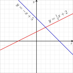
Two Graphs of linear equations in two variables

In mathematics, a linear equation is an equation that may be put in the form

a1x1+⋯+anxn+b=0,displaystyle a_1x_1+cdots +a_nx_n+b=0,

where x1,…,xndisplaystyle x_1,ldots ,x_n are the variables (or unknowns or indeterminates), and b,a1,…,andisplaystyle b,a_1,ldots ,a_n are the coefficients, which are often real numbers. The coefficients may be considered as parameters of the equation, and may be stated as arbitrary expressions, restricted to not contain any of the variables. To yield a meaningful equation for non-zero values of b,displaystyle b, the coefficients are required not to be all zeros.

In the words of algebra, a linear equation is obtained by equating to zero a linear polynomial over some field, where the coefficients are taken from, and that does not contain the symbols for the indeterminates.

The solutions of such an equation are the values that, when substituted to the unknowns, make the equality true.

The case of just one variable is of particular importance, and it is frequent that the term linear equation refers implicitly to this particular case, in which the name unknown for the variable is sensibly used.

All the pairs of numbers that are solutions of a linear equation in two variables form a line in the Euclidean plane, and every line may be defined as the solutions of a linear equation. This is the origin of the term linear for qualifying this type of equations. More generally, the solutions of a linear equation in n variables form a hyperplane (of dimension n – 1) in the Euclidean space of dimension n.

Linear equations occur frequently in all mathematics and their applications in physics and engineering, partly because non-linear systems are often well approximated by linear equations.

This article considers the case of a single equation with coefficients from the field of real numbers, for which one studies the real solutions. All its content applies for complex solutions and, more generally, for linear equations with coefficient and solutions in any field. For the case of several simultaneous linear equations, see System of linear equations.

One variable

Frequently the term linear equation refers implicitly to the case of just one variable. This case, in which the name unknown for the variable is sensibly used, is of particular importance, since it offers a unique value as solution to the equation. According to the above definition such an equation has the form

ax+b=0,displaystyle ax+b=0,

and, for a ≠ 0, a unique value as solution

x=−ba.displaystyle x=-frac ba.

The above equation may always be rewritten to

ax=−b=b′,displaystyle ax=-b=b',

and the solution is of course the same in both cases:

x=b′a=−ba.displaystyle x=frac b'a=-frac ba.

In the case of a=0displaystyle a=0, two possibilities emerge:

1. 
   b=0:displaystyle b=0: Every value for xdisplaystyle x is a solution to the equation 0⋅x+0=0,displaystyle 0cdot x+0=0, and


2. 
   b≠0:displaystyle bneq 0: There is no solution for the equation 0⋅x+b=0,displaystyle 0cdot x+b=0, the equation is said to be inconsistent.

Two variables

In the case of just two variables the indexed variable names x1displaystyle x_1 and x2displaystyle x_2 and the respective coefficients a1displaystyle a_1 and a2displaystyle a_2 are often replaced, for the convenience of not having to deal with indices, by xdisplaystyle x, ydisplaystyle y, adisplaystyle a and bdisplaystyle b, respectively. As a consequence, the so called constant term, named coefficient bdisplaystyle b in the above notation, must also be renamed; cdisplaystyle c suggests itself. A linear equation in two variables is then denoted as

ax+by+c=0.displaystyle ax+by+c=0.

Any change to such an equation that does not alter the set of solutions, i.e., the set of pairs (x,y)displaystyle (x,y), that satisfy this equation (i.e., make it an identity), generates an equivalent equation. It is immediate that changing the involved names (e.g. capitalizing names or using other letters) and also reordering the equation (e.g. by moving terms to the other side), does not change this set of solutions, and thus results in an equivalent equation, like, e.g.

Ax+By=C,displaystyle Ax+By=C,quad with A=a,B=bdisplaystyle quad A=a,;B=bquad and C=−c.displaystyle quad C=-c.

These equivalent variants are sometimes given generic names, like general form or standard form,^[1] but contribute no new concepts.

The set of solutions also does not change when both sides of the equation are multiplied by the same non-zero number. According to the above definition, adisplaystyle a and bdisplaystyle b (identically Adisplaystyle A and Bdisplaystyle B) are not both zero, so multiplying the equation by the reciprocal of one of these non-zero coefficients, results in an equivalent equation with +1displaystyle +1 as the coefficient of one variable. This variable can be isolated on the left hand side, leaving an expression, possibly containing the other variable on the right hand side. This leads to either

b≠0:y=mx+y0,displaystyle bneq 0:quad y=mx+y_0,quad ; with m=−abdisplaystyle quad m=-frac abquad ; and y0=−cb,displaystyle quad y_0=-frac cb,quad or

a≠0:x=m′y+x0,displaystyle aneq 0:quad x=m'y+x_0,quad with m′=−badisplaystyle quad m'=-frac baquad and x0=−ca.displaystyle quad x_0=-frac ca.

When both coefficients adisplaystyle a and bdisplaystyle b are not zero, then both forms exist, and, assuming real numbers as coefficients and for the domain of the variables, the set of solutions for both equations can then be denoted as

S=∀x∈R,displaystyle S=(x,mx+y_0),quad which is equal to the set S=∀y∈R.displaystyle quad S=(m'y+x_0,y).

In this case both components of the pairs in the set Sdisplaystyle S vary over all real numbers, thereby depending in a so called linear affine manner on the respective other.

When exactly one coefficient, either adisplaystyle a or bdisplaystyle b, is not zero, then one equation remains, which is either

y=y0,displaystyle y=y_0,quad for a=0,b≠0,displaystyle quad a=0,;bneq 0,quad with the set of solutions Sx=(x,y0),displaystyle quad S_x=;forall xin mathbb R ,quad or

x=x0,displaystyle x=x_0,quad for b=0,a≠0,displaystyle quad b=0,;aneq 0,quad with the set of solutions Sy=∀y∈R.displaystyle quad S^y=;forall yin mathbb R .

For both alternatives this is a set of pairs of numbers, where either the second component is a constant, and the first varies over all the reals (Sxdisplaystyle S_x), or the first is a constant, and the second varies over all the reals (Sydisplaystyle S^y).

In Cartesian coordinates

Every single solution of a linear equation in two variables can be interpreted as two coordinate values, fixing a point in the Euclidean plane with a Cartesian coordinate system. The sets of solutions of such an equation make up a two-dimensional graph, which can be depicted in this plane. Conventionally, the first component of a solution (x,y)displaystyle (x,y), the xdisplaystyle x-value, is assigned to a horizontally drawn xdisplaystyle x-axis, and the second component, the ydisplaystyle y-value, to a vertical ydisplaystyle y-axis.

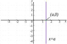
Vertical Line x=x0displaystyle x=x_0
(in the picture:x0↦a)displaystyle (textin the picture:;x_0mapsto a)

In the case of a≠0,b=0displaystyle aneq 0,;b=0 the equation is x=x0,displaystyle x=x_0, and the set of its solutions Sy=∀y∈Rdisplaystyle S^y=;forall yin mathbb R has a vertical line as its graph, as shown in the figure to the right. The value x0=−ca,displaystyle x_0=-tfrac ca, where the line intersects the xdisplaystyle x-axis in the point (x0,0)displaystyle (x_0,0), is called an xdisplaystyle x-intercept. Except for x0=0,displaystyle x_0=0, when the graph coincides with the ydisplaystyle y-axis, graphs of this kind do not intersect the ydisplaystyle y-axis, they have no ydisplaystyle y-intercept.

The set of solutions defines a function f(t)displaystyle f(t) and, simultaneously, the graph of this function, by interpreting the pairs (x,y)displaystyle (x,y) as (t,f(t)),displaystyle (t,f(t)), provided that any two such solutions that differ in their second value (y=f(t)displaystyle y=f(t)), also differ in their respective first values (x=tdisplaystyle x=t). The set Sy=∀y∈Rdisplaystyle S^y=;forall yin mathbb R violates this condition: all real values ydisplaystyle y in the second component have the same first component x0.displaystyle x_0. Nevertheless, a graph for this set may be drawn, but it is not a graph of a function under the conventional assignment of axes, it obviously fails the vertical line test. This is the only type of straight line which is not the graph of any function f(t)displaystyle f(t).

Horizontal Line y=y0displaystyle y=y_0
(in the picture:y0↦b)displaystyle (textin the picture:;y_0mapsto b)

The sets Sxdisplaystyle S_x and Sdisplaystyle S satisfy the above condition, and the graph of Sx=(x,y0)displaystyle S_x=;forall xin mathbb R is shown to the right. In this case of a=0,b≠0displaystyle a=0,;bneq 0 the graph of the constant function f(x)=y=y0displaystyle f(x)=y=y_0 is a horizontal line. The value y0=−cb,displaystyle y_0=-tfrac cb, where the line intersects the ydisplaystyle y-axis, is called ydisplaystyle y-intercept. Except for y0=0,displaystyle y_0=0, where the graph coincides with the xdisplaystyle x-axis, graphs of this kind have no xdisplaystyle x-intercept.

In the case of a≠0≠bdisplaystyle aneq 0neq b with the equation y=mx+y0displaystyle y=mx+y_0 the set of solutions is S=∀x∈R.displaystyle S=(x,mx+y_0). It consists of pairs of numbers, with the first component varying over all the reals, and the other being calculated by a simple expression, representing a linear map (x↦mxdisplaystyle xmapsto mx) and adding a constant (y0displaystyle y_0). This is sometimes called a linear affine function, or simply also linear function, slightly abusing the strict term linear. Also in this case the graph of a linear equation in two variables is a straight line (see figure at the top) that intersects the xdisplaystyle x-axis at xdisplaystyle x-intercept x0=−cadisplaystyle x_0=-tfrac ca (i.e., (x0,0)displaystyle (x_0,0) is a solution) and the ydisplaystyle y-axis at the ydisplaystyle y-intercept y0=−cbdisplaystyle y_0=-tfrac cb (i.e., (0,y0)displaystyle (0,y_0) is a solution).

Besides the intercepts being obvious from graphing the solutions of a linear equation in two variables, also their ratio (if it exists) can be graphically interpreted as determining the incline of the considered line (and all lines parallel to it). The slope of a straight line, usually introduced as rise over run, is the negative ratio of the rise, the ydisplaystyle y-intercept, to the run, the xdisplaystyle x-intercept. The negative sign accommodates for a positive slope, when the line rises for increasing xdisplaystyle x-values. Immediately

−y0x0=−−cb−ca=−ab=m,displaystyle -frac y_0x_0=-frac -tfrac cb-tfrac ca=-frac ab=m,

which holds if both intercepts exist. If the xdisplaystyle x-intercept does not exist (a=0displaystyle a=0), the slope mdisplaystyle m equals 0,displaystyle 0, belonging to a horizontal line.

Since rise and run of a straight line can be determined not only between the intercept points and the origin (x0−0displaystyle x_0-0 and y0−0displaystyle y_0-0), but also between arbitrary points (x1,y1)displaystyle (x_1,y_1) and (x2,y2)displaystyle (x_2,y_2) on the line, the slope may also be determined by

m=y2−y1x2−x1=y1−y2x1−x2.displaystyle m=frac y_2-y_1x_2-x_1=frac y_1-y_2x_1-x_2.

Denoting the angle enclosed by the xdisplaystyle x-axis and the line as φ,displaystyle varphi , then

tan⁡φ=m=−ab.displaystyle tan varphi =m=-frac ab.

For b=0displaystyle b=0 the slope is undefined (φ=π/2displaystyle varphi =pi /2).

This shows that only two of x0,y0displaystyle x_0,;y_0 and mdisplaystyle m can be selected independently.

With the premise that at least one axis is intersected, and since both intercept values may range over the whole real number line, all parallels to both axes as well as all oblique straight lines, i.e., in fact all straight lines in the Euclidean plane, can be expressed by linear equations in two variables, and all such equations denote either oblique or axis-parallel straight lines. Therefore all equations, equivalent to one of the above forms are often referred to as "equations of a line". They are adjusted to fit best to specific tasks, and are given therefore specific names, described below. In what follows, x,y,t,θdisplaystyle x,;y,;t,;theta are the names of variables, and other letters denote constants (fixed numbers) as coefficients.

Slope–intercept form

This form relies on the habit of writing y=f(x)displaystyle y=f(x) and the conventional way of assigning the variables of the linear equation to the axes of a Cartesian coordinate system, drawn in the conventional manner as described above. This form exists only for b≠0,displaystyle bneq 0, allowing to isolate ydisplaystyle y on the left hand side

y=mx+y0.displaystyle y=mx+y_0.

This way the slope m=−abdisplaystyle m=-tfrac ab describes the inclination of the straight line which is the graph of this equation. The slope is positive for a line ascending to the right and negative, if the line ascends to the left. A zero-slope m=0displaystyle m=0 belongs to a horizontal line.

The ydisplaystyle y-intercept y0=−cbdisplaystyle y_0=-tfrac cb fixes the point (0,y0),displaystyle (0,y_0), where the line crosses the ydisplaystyle y-axis, and y0=0displaystyle y_0=0 characterizes lines that cross the origin (0,0).displaystyle (0,0).

Recalling the xdisplaystyle x-intercept as x0=−ca,displaystyle x_0=-tfrac ca, the above slope-intercept form, employing the slope mdisplaystyle m and the ydisplaystyle y-intercept, can be transformed to

y=−abx−cb=−ab(x+ba⋅cb)=m(x−x0),displaystyle y=-frac abx-frac cb=-frac ab(x+frac bacdot frac cb)=m(x-x_0),

involving the slope mdisplaystyle m and the xdisplaystyle x-intercept x0displaystyle x_0.

In the case of b=0,displaystyle b=0, there is no slope-intercept form in the above way, because a slope does not exist for φ=π/2displaystyle varphi =pi /2.

For a≠0≠bdisplaystyle aneq 0neq b it is possible to express the inverse functions f−1displaystyle f^-1 in the slope-intercept form as

x=m′y+x0,displaystyle x=m'y+x_0,quad with m′=ba.displaystyle m'=tfrac ba.

The graph of this equation, having the same set of solutions, is necessarily identical to the above graph, but depicting it under exchanged assignment of the variables to the coordinate-axes ((x,y)↦(y-axis,x-axis)displaystyle (x,y)mapsto (ytext-axis,;xtext-axis)), yields the usual f−1displaystyle f^-1-graph for inverse functions, the fdisplaystyle f-graph mirrored along y=x.displaystyle y=x. This holds for both (a=0,b≠0)displaystyle (a=0,;bneq 0) and (b=0,a≠0).displaystyle (b=0,;aneq 0).

The graph of a vertical line (b=0displaystyle b=0) with no existing slope and the equation x=ddisplaystyle x=d changes under this inverted assignment to the graph of the function y=ddisplaystyle y=d with zero-slope (ddisplaystyle d an arbitrary constant), and vice versa.

Point–slope form

It is observational evident that fixing an arbitrary point on a line and a slope uniquely defines this straight line. In the slope-intersect form this point on the line is either taken as the intersection (0,y0)displaystyle (0,y_0) with the ydisplaystyle y-axis, or the intersection (x0,0)displaystyle (x_0,0) with the xdisplaystyle x-axis and is combined with the slope mdisplaystyle m, provided its existence, to establish the equation for the according line. Generalizing this approach to an arbitrary point with coordinates (x1,y1)displaystyle (x_1,y_1) yields:

y−y1=m(x−x1).displaystyle y-y_1=m(x-x_1).

The point-slope form expresses the fact that the difference of the ydisplaystyle y coordinates between two points on a line (i.e., y−y1displaystyle y-y_1) is proportional to the difference of the xdisplaystyle x-coordinate (i.e., x−x1displaystyle x-x_1), with the proportionality constant m,displaystyle m, the slope of the line.

Intercept form

Straight lines that cross both coordinate axis outside the origin can be specified via the intercept form, that employs just these two values to specify an appropriate equation

xx0+yy0=1.displaystyle frac xx_0+frac yy_0=1.

The intercept form results from moving cdisplaystyle c in the equation ax+by+c=0displaystyle ax+by+c=0 to the right side, and then multiplying both sides of the equation with −1/c,displaystyle -1/c, yielding

(−ac)x+(−bc)y=1x0x+1y0y=1,displaystyle (-frac ac)x+(-frac bc)y=frac 1x_0x+frac 1y_0y=1,

which is identical to the above form. The intercept form also works conveniently in higher dimensions for specifying (hyper)planes, when their intersections with all coordinate axes exist and are known.

Two-point form

Two points (x1,y1)displaystyle (x_1,y_1) and (x2,y2)displaystyle (x_2,y_2) with x1≠x2displaystyle x_1neq x_2 (no vertical lines!) determine the slope of the line through these points. This slope, calculated as above, can be used with either point to employ the point-slope form, thereby establishing appropriate equations for this line, based on two points with different xdisplaystyle x-values. This yields

y−yj=y2−y1x2−x1(x−xj),displaystyle y-y_j=frac y_2-y_1x_2-x_1(x-x_j),quad for j=1,2.displaystyle j=1,2.

In the rest of this paragraph j=1displaystyle j=1 is used.

Expanded form

Expanding, regrouping, and appropriately factoring the products leads to

(y1−y2)x+(x2−x1)y+(x1y2−x2y1)=0,displaystyle (y_1-y_2)x+(x_2-x_1)y+(x_1y_2-x_2y_1)=0,

identifying: a=(y1−y2),b=(x2−x1),displaystyle quad a=(y_1-y_2),quad b=(x_2-x_1),quad and c=(x1y2−x2y1).displaystyle quad c=(x_1y_2-x_2y_1).

Symmetric form

Multiplying both sides of the 2-point form by (x2−x1)displaystyle (x_2-x_1) yields an equation in a symmetric form

(x2−x1)(y−y1)=(y2−y1)(x−x1).displaystyle (x_2-x_1)(y-y_1)=(y_2-y_1)(x-x_1).

This form also works in the case of a non-existing slope (x1=x2displaystyle x_1=x_2), but requires y1≠y2displaystyle y_1neq y_2 in this case: it correctly delivers x=x1.displaystyle quad x=x_1.

Determinant form

The products in the above equation result also from the evaluation of a 2-rowed determinant, inducing this form of the linear equation:

|x−x1y−y1x2−x1y2−y1|=0.displaystyle beginvmatrixx-x_1&y-y_1\x_2-x_1&y_2-y_1endvmatrix=0.

Mnemonic determinant

The products on the left hand side of the expanded version can be reproduced by evaluating the 3-rowed determinant, designed for easy memorability:

|xy1x1y11x2y21|=0.displaystyle beginvmatrixx&y&1\x_1&y_1&1\x_2&y_2&1endvmatrix=0.

Vectorial treatment

Any pair of numbers (x,y)displaystyle (x,y) may be treated as a vector, given by two components with respect to a Cartesian coordinate system. A (naive) vector starts at the origin (0,0)displaystyle (0,0), and ends at the given coordinates. Any two non-collinear vectors (a1,a2)displaystyle (a_1,a_2) and (b1,b2)displaystyle (b_1,b_2) span a parallelogram, with these three points. The area Adisplaystyle A of this parallelogramm can be calculated as the magnitude of the exterior product (2dim-cross product, geometric product, ...) of these vectors. In components this can be done by evaluating the absolute value of a determinant with the components:

A=||a1a2b1b2||..

Two given points P1=(x1,y1),P2=(x2,y2)displaystyle P_1=(x_1,y_1),;P_2=(x_2,y_2) and an arbitrary third point P=(x,y)displaystyle P=(x,y) are on one straight line (collinear), if, e.g., the vector from P1displaystyle P_1 to P2displaystyle P_2 and the vector from P1displaystyle P_1 to Pdisplaystyle P span no parallelogram, i.e., a parallelogram with area zero, i.e., also the vectors are collinear.

The vector from point P1displaystyle P_1 to point P2displaystyle P_2 can be expressed as

P12=P2−P1=(x2,y2)−(x1,y1)=(x2−x1,y2−y1)displaystyle P_12=P_2-P_1=(x_2,y_2)-(x_1,y_1)=(x_2-x_1,y_2-y_1)

and similarly the vector from point P1displaystyle P_1 to an arbitrary point Pdisplaystyle P is

P1.=P−P1=(x,y)−(x1,y1)=(x−x1,y−y1).displaystyle P_1.=P-P_1=(x,y)-(x_1,y_1)=(x-x_1,y-y_1).

Equating the exterior product of these two vectors, as specified above, to zero, yields a linear equation

|x−x1y−y1x2−x1y2−y1|=0,displaystyle beginvmatrixx-x_1&y-y_1\x_2-x_1&y_2-y_1endvmatrix=0,

which is identical to the determinant form above.

Matrix form

Writing a linear equation in two unknowns in the form

Ax+By=C,displaystyle Ax+By=C,

and considering the collection of coefficients (A,B)displaystyle (A,B) as a (1,2)displaystyle (1,2)-matrix, and the collection of variables (xy)displaystyle beginpmatrixx\yendpmatrix as a (2,1)displaystyle (2,1)-matrix, then their matrix product equals the (1,1)displaystyle (1,1)-matrix (C):displaystyle beginpmatrixCendpmatrix:

(AB)(xy)=(C).displaystyle beginpmatrixA&Bendpmatrixbeginpmatrixx\yendpmatrix=beginpmatrixCendpmatrix.

This notation can easily expanded to more linear equations in more than two variables. For example, a system of two equations in two variables

A1x+B1y=C1,displaystyle A_1x+B_1y=C_1,,

A2x+B2y=C2,displaystyle A_2x+B_2y=C_2,,

can be denoted with a (2,2)displaystyle (2,2)-matrix and a (2,1)displaystyle (2,1)-matrix for the coefficients, by equaling the matrix product of the (2,2)displaystyle (2,2)-coefficient matrix with the (2,1)displaystyle (2,1)-variable matrix to the (2,1)displaystyle (2,1)-matrix of the constant terms:

(A1B1A2B2)(xy)=(C1C2).displaystyle beginpmatrixA_1&B_1\A_2&B_2endpmatrixbeginpmatrixx\yendpmatrix=beginpmatrixC_1\C_2endpmatrix.

A system of three linear equations in four variables would employ a (3,4)displaystyle (3,4)-matrix for the coefficients of the variables, which, multiplied with the (4,1)displaystyle (4,1)-(column)-matrix of the variables, is equaled to the (3,1)displaystyle (3,1)-matrix of the constant terms. For this ready extendability to higher dimensions, the matrix notation is a common representation tool for a system of linear equations, in linear algebra, and in computer programming. There are named methods for solving systems of linear equations, like Gauss-Jordan which can be expressed in matrix elementary row operations.

Parametric form

The parametric form of a curve is useful to e.g. describe the movement of a point along this curve, and controlling this movement with a single parameter. This setting resembles the task in physics, where a particle starts at time t=0displaystyle t=0 at some point in space, say (h,k)displaystyle (h,k), and travels along the curve, where it reaches point (p,q)displaystyle (p,q) at time t=1.displaystyle t=1. With linear equations the curves are restricted to straight lines.

This task can be solved by adding a motion from h→pdisplaystyle hto p in the direction of the xdisplaystyle x-axis and a simultaneous motion from k→qdisplaystyle kto q in the direction of the ydisplaystyle y-axis, both motions controlled by the parameter t.displaystyle t. The motion in xdisplaystyle x-direction can be described as

x=(k−h)t+hdisplaystyle x=(k-h)t+h

and similarly, the motion in xdisplaystyle x-direction can be described as

y=(q−k)t+k.displaystyle y=(q-k)t+k.

These two linear equations, with variables (t,x)displaystyle (t,x) and (t,y)displaystyle (t,y), make up a parametric form for a linear equation with variables (x,y)displaystyle (x,y) that can be constructed from the two-point form with (h,k)displaystyle (h,k) and (p,q)displaystyle (p,q) as points.

For t=0:(x,y)|t=0=(h,k)displaystyle t=0:quad (x,y) and for t=1:(x,y))|t=1=(p,q).displaystyle t=1:quad (x,y)) For all tdisplaystyle t in the interval [0,1]displaystyle [0,1] the point (x,y)|tdisplaystyle (x,y) is on the straight line segment connecting the points for t=0displaystyle t=0 and t=1.displaystyle t=1. This is sometimes called interpolation. For values of tdisplaystyle t outside this interval, points outside of the segment, but still on the line are addressed extrapolation.

Connection with linear functions

A linear equation, written in the form y = f(x) whose graph crosses the origin (x,y) = (0,0), that is, whose y-intercept is 0, has the following properties:

• 
  Additivity: f(x1+x2)=f(x1)+f(x2) displaystyle f(x_1+x_2)=f(x_1)+f(x_2)
  


• 
  Homogeneity of degree 1: f(ax)=af(x),displaystyle f(ax)=af(x),,
  

where a is any scalar. A function which satisfies these properties is called a linear function (or linear operator, or more generally a linear map). However, linear equations that have non-zero y-intercepts, when written in this manner, produce functions which will have neither property above and hence are not linear functions in this sense. They are known as affine functions.

Example

An everyday example of the use of different forms of linear equations is computation of tax with tax brackets. This is commonly done with a progressive tax computation, using either point–slope form or slope–intercept form.

More than two variables

For the general case of a linear equation with n>2displaystyle n>2 unknowns the equation may always be assumed to be be denoted as at the top

a1x1+a2x2+⋯+anxn+b=0.displaystyle a_1x_1+a_2x_2+cdots +a_nx_n+b=0.

Sometimes bdisplaystyle b is called the absolute term, and the term coefficient is reserved for the ai.displaystyle a_i. A variant to denote b,displaystyle b, stemming from the use in polynomials, is to write a0displaystyle a_0 instead, alluding to the zeroth power of any variable, that always reduces to 1.displaystyle 1.

When dealing with n=3displaystyle n=3 variables, it is common to use x,ydisplaystyle x,;y and zdisplaystyle z instead of indexed variables.

The set of solutions of such an equation is a set of ndisplaystyle n-tuples, and each ndisplaystyle n-tuple makes the equation an identity, when its components are inserted for the respective unknowns. The values of the variables with zero coefficients are taken arbitrarily from the field of coefficients.

For an equation to have meaningful solutions, at least one coefficient must be non-zero. This can be formulated as

a12+a22+⋯+an2=∑i=1nai2>0.displaystyle a_1^2+a_2^2+cdots +a_n^2=textstyle sum _i=1^na_i^2>0.

If all coefficients aidisplaystyle a_i equal zero, then, as mentioned for one variable, the equation is either inconsistent (for b≠0displaystyle bneq 0) and there is no solution, or all
ndisplaystyle n-tuples are solutions.

The set of solutions (ndisplaystyle n-tuples) of a linear equation in ndisplaystyle n variables is an (n−1)displaystyle (n-1)-dimensional hyperplane in an ndisplaystyle n-dimensional Euclidean space (or affine space if the coefficients are complex numbers or belong to any field). Within the usual setting of real numbers and a three-dimensional space with Cartesian coordinates, the set of the solutions of a linear equation with three variables describes a plane in the intuitive sense.

A given equation may be solved for all variables with a non-zero coefficient. Let jdisplaystyle j be an index such that aj≠0,displaystyle a_jneq 0, then

xj=−(baj+a1ajx1+⋯+0⋅xj+⋯+anajxn).displaystyle x_j=-(tfrac ba_j+tfrac a_1a_jx_1+cdots +0cdot x_j+cdots +tfrac a_na_jx_n).

This way the linear equation can be seen as defining a function of (n−1)displaystyle (n-1) variables, which maps, assuming the setting of reals, the set of (n−1)displaystyle (n-1)-tuples^[2] of reals to the real numbers, i.e.:

xj:Rn−1→Rdisplaystyle x_j:;mathbb R ^n-1to mathbb R

See also

• Line (geometry)


• Linear function


• Linear equation over a ring


• Algebraic equation


• Linear belief function


• Linear inequality

Notes

References

• 
  Barnett, R.A.; Ziegler, M.R.; Byleen, K.E. (2008), College Mathematics for Business, Economics, Life Sciences and the Social Sciences (11th ed.), Upper Saddle River, N.J.: Pearson, ISBN 0-13-157225-3.mw-parser-output cite.citationfont-style:inherit.mw-parser-output qquotes:"""""""'""'".mw-parser-output code.cs1-codecolor:inherit;background:inherit;border:inherit;padding:inherit.mw-parser-output .cs1-lock-free abackground:url("//upload.wikimedia.org/wikipedia/commons/thumb/6/65/Lock-green.svg/9px-Lock-green.svg.png")no-repeat;background-position:right .1em center.mw-parser-output .cs1-lock-limited a,.mw-parser-output .cs1-lock-registration abackground:url("//upload.wikimedia.org/wikipedia/commons/thumb/d/d6/Lock-gray-alt-2.svg/9px-Lock-gray-alt-2.svg.png")no-repeat;background-position:right .1em center.mw-parser-output .cs1-lock-subscription abackground:url("//upload.wikimedia.org/wikipedia/commons/thumb/a/aa/Lock-red-alt-2.svg/9px-Lock-red-alt-2.svg.png")no-repeat;background-position:right .1em center.mw-parser-output .cs1-subscription,.mw-parser-output .cs1-registrationcolor:#555.mw-parser-output .cs1-subscription span,.mw-parser-output .cs1-registration spanborder-bottom:1px dotted;cursor:help.mw-parser-output .cs1-hidden-errordisplay:none;font-size:100%.mw-parser-output .cs1-visible-errorfont-size:100%.mw-parser-output .cs1-subscription,.mw-parser-output .cs1-registration,.mw-parser-output .cs1-formatfont-size:95%.mw-parser-output .cs1-kern-left,.mw-parser-output .cs1-kern-wl-leftpadding-left:0.2em.mw-parser-output .cs1-kern-right,.mw-parser-output .cs1-kern-wl-rightpadding-right:0.2em
  

External links

• 
  Linear Equations and Inequalities Open Elementary Algebra textbook chapter on linear equations and inequalities.


• 
  Hazewinkel, Michiel, ed. (2001) [1994], "Linear equation", Encyclopedia of Mathematics, Springer Science+Business Media B.V. / Kluwer Academic Publishers, ISBN 978-1-55608-010-4